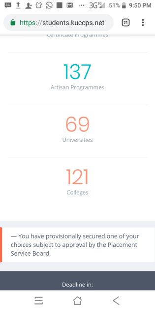
Category Archives: Latest Education News

A category dedicated to all education news in Kenya and other countries across the world. This is your one stop location for all news related to the education sector.

Kuccps list of Courses offered at GRETSA University; Course Codes, Fees, Requirements, Cluster Cut Off Points

Kuccps list of Courses offered at GRETSA University; Course Codes, Fees, Requirements, Cluster Cut Off Points

GRETSA UNIVERSITY

PROGRAMMES ON OFFER FOR 2023/2024 CYCLE

# PROGRAMME CODE PROGRAMME NAME INSTITUTION TYPE YEAR 1 – PROGRAMME COST 2023/2024 CUTOFF 2020 CUTOFF
1 1088115 BACHELOR OF SCIENCE IN COMPUTER SCIENCE KSH 140,000 19.223 25.737
2 1088133 BACHELOR OF COMMERCE KSH 132,000 22.544 22.361
3 1088135 BACHELOR OF EDUCATION (ARTS) KSH 130,000 22.636 26.953
4 1088171 BACHELOR OF ARTS IN COMMUNITY DEVELOPMENT KSH 130,000 22.926 24.373
5 1088221 BACHELOR OF SCIENCE (HOSPITALITY AND TOURISM MANAGEMENT) KSH 152,000
6 1088224 BACHELOR OF SCIENCE IN HOSPITALITY MANAGEMENT KSH 152,000 23.610 22.361

Schools’ Nemis Portal replaced by Kemis

Schools’ portal Nemis replaced by Kemis

A multi-agency team tasked with consolidating existing registers for all students in schools, ranging from foundation learning to university level, to a single database was unveiled today.

The team, which brings together State agencies led by the Ministry of Education, development partners, technology providers and other stakeholders, will set up the Kenya Education Management Information System (KEMIS) to replace the current NEMIS which has been criticised for inefficiencies.

Basic Education PS Prof Julius Bitok said the piloting of KEMIS will be launched in July this year ahead of full transitioning in September.

He explained that the envisaged KEMIS will create an integrated database that will be relied upon to guide education planning and the allocation of relevant resources.

Parents and other stakeholders will also be able to access KEMIS through a mobile phone based application.

“The rollout of KEMIS marks a critical milestone in ensuring that data-driven decision making becomes the cornerstone of education planning and service delivery in Kenya.”

He said KEMIS will also make it impossible to manipulate capitation amounts by registering ghost schools and inflating school populations.

“By consolidating all learner data, from ECDE to higher education, into one platform, the system will enhance accuracy, transparency, and accessibility. It will ensure the government has the right statistics on every school to inform the distribution of teachers, capitation, books and other resources.”

KEMIS will address longstanding challenges in separate registration databases for education levels: Early Childhood and Development Education (ECDE), basic education, TIVETS and universities. It will also consolidate and store data for students, teachers, and institutions.

It will also address emerging issues such as data security and privacy and provide a platform for real-time access to data, enabling monitoring, evaluation and analytics on education transitions and other variables.

Immigration and Citizen Services PS Dr. Belio Kipsang said KEMIS will also be integrated with the births and deaths register through the Civil Registration Services and the National Registration Bureau to provide a unique personal number for every learner.

“Under the Maisha ecosystem, we will provide a Unique Personal Identifier (UPI) to every newborn, which will also be used by KEMIS. In the event of death, the UPI will be the death certificate number. This will help us with accurate data on inevitable transitions.”

Members of Parliament, led by Education Committee Chairman Julius Melly, stated that KEMIS will be a useful platform for guiding budget estimates.

“Whoever has accurate data is well placed to make appropriate decisions on budget allocation. We shall support the Ministry’s legislative agenda in Parliament to ensure this transformative system is fully backed by law.”

The statement comes in the wake of uproar by MPs following massive slashing of the Education budget by the National Treasury resulting in zero allocations for national exams and KEMIS. Besides the Tinderet MP, Mary Emaase (Teso South), Phyilis Bartoo (Moiben) and Joseph Makilap (Baringo North) also witnessed the unveiling of the 15-member team.

Also present was ICT PS Eng. John Tanui, whose Department will play a key role through the Konza Technopolis Development Authority and teachers’ union representatives led by KNUT Secretary General Collins Oyuu.

Free grade 3 schemes of work; Download them here for free

Are you in need of free grade 3 schemes of work? You can now download all the grade 3 schemes of work here at no cost. Schemes of work is one of the many professional documents that a teacher must have.

FREE GRADE 3 SCHEMES OF WORK.

TERM TWO SCHEMES

Get the schemes below at no cost;

[embeddoc url=”https://educationnewshub.co.ke/wp-content/uploads/2020/12/GRADE-THREE-CRE-SCHEME-OF-WORK-TERM-TWO.pdf”]

Click here for a free download of the schemes of work.

[embeddoc url=”https://educationnewshub.co.ke/wp-content/uploads/2020/12/ENVIRONMENTAL-SCHEME-GRADE-THREE-TERM-TWO.pdf”]

Click here for a free download of the schemes of work.

[embeddoc url=”https://educationnewshub.co.ke/wp-content/uploads/2020/12/MATHEMATICS-GRADE-THREE-SCHEME-OF-WORK-TERM-TWO.pdf”]

Click here for a free download of the schemes of work.

[embeddoc url=”https://educationnewshub.co.ke/wp-content/uploads/2020/12/MAAZIMIO-YA-KAZI-YA-KISWAHILI-MUHULA-WA-PILI.pdf”]

Click here for a free download of the schemes of work.

[embeddoc url=”https://educationnewshub.co.ke/wp-content/uploads/2020/12/GRADE-THREE-MUSIC-SCHEME-OF-WORK-TERM-TWO.pdf”]

Click here for a free download of the schemes of work.

[embeddoc url=”https://educationnewshub.co.ke/wp-content/uploads/2020/12/GRADE-THREE-MOVEMENT-SCHEME-OF-WORK-TERM-TWO.pdf”]

Click here for a free download of the schemes of work.

[embeddoc url=”https://educationnewshub.co.ke/wp-content/uploads/2020/12/GRADE-THREE-HYGIENE-AND-NUTRITION-SCHEME-TERM-TWO.pdf”]

Click here for a free download of the schemes of work.

[embeddoc url=”https://educationnewshub.co.ke/wp-content/uploads/2020/12/GRADE-THREE-ENGLISH-SCHEME-OF-WORK-TERM-TWO.pdf”]

Click here for a free download of the schemes of work.

Didn’t find what you were looking for? Worry not. Get all primary and secondary materials here.

Moi University – KUCCPS Students Admission Letters and Lists Portal

Moi University – KUCCPS Students Admission Letters and Lists Portal

The Moi University Kuccps Admission Letter is an important document that you need in order to prepare for first year reporting.

How To Download your Moi University Admission Letter

Government Sponsored Students (placed by KUCCPS)

NBBefore proceeding, ensure you have received an SMS from KUCCPS or Moi University indicating your placement to Moi University. You can also confirm you placement from your KUCCPS portal.

Requirements to download the letter

Digital passport photo (yellow background), scanned copies of National ID card, Birth certificate, KCSE Results slip and high school leaving certificate.

1. First ensure you have received an invitation to Moi University from KUCCPS. View the Moi University KUCCPS List here.

2. Login via the Admission Portal using the following link: https://admissions.mu.ac.ke/gsp/login-kuccps

3. Key in the required login details in the following format: KCSE Index number/year and click Login. i.e., if your index number is 44445678 then key in this format 44445678/2022 where 44445678 is your index number and Year is the year you sat for your Kenya Certificate of Secondary Education (KCSE). Remember to provide the Security Stamp as requested.

4. The first time you login, you are required to ACCEPT or REJECT the Programme you have been offered. Accepting the offer gives you access to other services while rejecting denies you access to any other services.

5. Fill in the required registration details and download your admission letter

Self Sponsored Students

1. Click the following link: https://admissions.mu.ac.ke/ssp/admission-letter and proceed as instructed

To Apply for admission, first view here the Programmes and Admission requirements; then proceed to apply online here.

Enquiries
Further enquiries can be made through

Email:  admissions@mu.ac.ke or directorict@mu.ac.ke or ict@mu.ac.ke

OR

SMS/Call/WhatsApp:

Main Campus: 0724 288 774

College of Health Sciences: 0724 950 422

Nairobi Campus: 0724 316 144

Coast Campus: 0724 856 135

Continue reading:

Your Complete guide to Higher Education Courses:

Alliance High School KCSE Results 2020/2021- Whole school results analysis

ALLIANCE BOYS HIGH SCHOOL KCSE 2020/2021 RESULTS ANALYSIS (SCHOOL MEAN, INDIVIDUAL CANDIDATES’ RESULTS AND MEAN GRADE SUMMARY)- The Alliance High School (or AHS) popularly known as “Bush”, is a public national high school for boys located in Kikuyu, Kiambu, Kenya. The school posts impressive performance in the KCSE exams, every year.

Related news; How to get the KCSE 2020/2021 results via Knec SMS Code and online portal

ALLIANCE BOYS HIGH SCHOOL’S KCSE 2019 RESULTS

In 2019 KCSE examination resultsAlliance High School a national school, posted a sturning school mean of 10.019 to emerge the top best school in Kiambu County and 4th overall best nationally.

Here is the KCSE 2019 results distribution of grades for Alliance High School;

ALLIANCE HIGH SCHOOL KCSE RESULTS 2019
Grade Entry
A 48
A- 160
B+ 95
B 56
B- 26
C+ 21
C 8
C- 8
D+ 1


Read more details here; KCSE 2019 list of top 200 schools nationally; Full list.

You may also like; KCSE 2019 national results and ranking per subject- Physics

ALLIANCE BOYS HIGH SCHOOL KCSE 2020 RESULTS ANALYSIS MEAN GRADE SUMMARY

Looking for KCSE 2020/2021 results for all schools and candidates? Visit this portal; KCSE RESULTS PORTAL.

The school registered a total of 398 candidates in the KCSE 2020 exam. In the just released KCSE 2020 results, the school posted an impressive mean score of _ . The good news is that_ candidates managed to score above C+ (plus), which is the minimum university entry grade. This translates to a percentage of _% securing direct entry to university under the placement body, KUCCPS.

Download KCSE 2020/2021 results for this school here; Official Knec KCSE Results Portal

Here is a complete distribution of grades for the school in KCSE 2020 results;

KCSE RESULTS 2020
Grade Entry
A
A-
B+
B
B-
C+
C
C-
D+
D


You may also like; Alliance Girls’ High School; KCSE results analysis, contacts, location, Admission Letters and more

Bachelor of Science in Cyber Security and Digital Forensics Kuccps Course requirements, fees and duration

Bachelor of Science in Cyber Security and Digital Forensics

Duration: 4 Years

Start Date: 

Cost: KES 105,000 per year

Mode of Delivery: Online

Application Due: Open

Fee Structure and Payment

Overview

The Bachelor of Science in Cyber Security and Digital Forensics program is meticulously designed to equip learners with the knowledge, skills, and attitudes required to address the ever-evolving landscape of cyber threats. Its primary goal is to provide comprehensive protection to digital, computer, and online assets of organizations. The curriculum remains adaptable and responsive to emerging trends in cyber security and digital forensics, guided by a commitment to open learning and the removal of barriers that impede knowledge dissemination. 

Cyber Security Career Projections:

Graduates of this program can pursue various rewarding careers, including but not limited to:

  • Cybersecurity Analyst
  • Information Security Specialist
  • Security Administrator
  • Forensic Analyst
  • Blockchain Security Expert
  • Cloud Security Specialist

Programme Structure

Upon successful completion of this program, learners will demonstrate the ability to:

  • Proficiently identify cybersecurity risks and vulnerabilities in diverse digital environments.
  • Conduct digital forensics investigations using industry-standard tools, methodologies, and ethical standards.
  • Implement comprehensive security measures to safeguard an organization’s ICT assets against both external and internal threats.
  • Develop and enact robust cybersecurity and digital forensics policies and strategies aligned with industry best practices. 

Programme Learning Outcomes

By the end of this programme, the student will be able to:

  1. Identify cyber security risks and vulnerabilities.
  2. Perform digital forensics using appropriate tools, techniques and standards.
  3. Protect an organization’s ICT assets from external and internal attacks.
  4. Develop cybersecurity and digital forensics policies and strategies.

Total credit hours and course units required for graduation

Total credit hours and course units required for graduation The programme shall be offered in 8 semesters. The minimum total courses for the programme are 48. The minimum total course credit hours required for graduation is 144 hours.

Admission Requirements

A candidate must satisfy the general University admission criteria for undergraduate programmes.

  1. A mean grade of C+ and above at KCSE OR
  2. Diplomas or professional qualifications OR
  3. A certificate of foundation or bridging courses from recognised institutions OR
  4. A portfolio for the purpose of recognition of prior learning OR
  5. Kenya Advanced Certificate of Education with a minimum of 1 principal OR
  6. A bachelor’s degree from an institution recognised by Senate.

Regulations On Credit Accumulation And Transfer

Credit Accumulation

Regulations on credit accumulation, including possible pathways, shall be in line with the provisions of Universities Regulations, Universities Standards and Guidelines, and general national trends.

Credit Transfer

A candidate may be allowed to transfer credits from part or all of the coursework requirements if the senate is satisfied that the candidate has completed and passed the prescribed courses(s) at the undergraduate level from accredited institutions and programs recognized by the senate. Any course considered for credit transfer must have been completed at an equivalent level and in an equivalent institution, with a minimum grade of 50%.

Guidelines For Transfer Of Credit/ Exemptions

A candidate may be exempted from degree level courses if the Senate is satisfied that the candidate has completed a similar course at the Diploma level from a recognized institution. The general rules governing credit transfers and exemptions will apply. In addition, the following rules apply:

  1. Must meet the requirements for admission to the Bachelor of Data Science program.
  2. Must obtain and submit an official transcript from the previous university/college indicating academic status, courses offered, credits units completed, and grades obtained.
  3. Will be allowed to transfer/exempt credits earned from the courses described, but only up to 49%.
  4. If permitted to transfer/exempt, he/she will not be permitted to transfer units in courses in which he/she received a pass mark of less than 50%.
  5. All applications must be accompanied by recommendations from the institution from which he or she is transferring.
  6. The school will evaluate the application and make recommendations to the Sen- ate.

Student Assessment Levels

Student Assessment at programme level

The course will be assessed through:

  1. Content embedded quizzes
  2. Online practical work
  3. Open book tests
  4. Project reports
  5. End of course online examination

The projects will be assessed through e- portfolios. Students will present their work to an evaluation panel. All students’ work will be checked for plagiarism. The students should be logged in with the university provided login details in order to carry out any task.

Countinous Assessment

Tests/Tasks: 50%

Examination 50%

Programme Courses

FIRST SEMESTER SECOND SEMESTER
Introduction to Computer Systems Computer Networks
Database systems Computer Architecture
Differential and Integral Calculus Physics for Computing Systems and Digital Electronics
Introduction to Programming Psychology
Digital Markets Architecture Mathematics for cybersecurity and digital forensics
Introduction to Cybersecurity and Digital Forensics Discrete Mathematics
IoT and Security Assembly Language

More articles with related information on KUCCPS

Kuccps opens portal for 2024/2025 applications by KCSE 2023 students

KUCCPS Student portal login student.kuccps.net for Admission Application
How to check kuccps degree and diploma placement
Kuccps admission lists and letters pdf for all universities (How to download Kuccps letter)
Kuccps Diploma Programmes (Course codes, requirements and institutions)
Kuccps cut off points for all courses
Kuccps cutoff points 2024
KUCCPS opens portal for first application, revision of courses for KCSE 2023 candidates
Kuccps opens student portal for University and College placement applications/ revision of courses 2024
KUCCPS latest placement news for KCSE 2023 candidates- CS Magoha speaks
kuccps placement 2024 (How to get results and admission letters)
Kuccps latest news 2024 (How to apply for Courses, Revise, Check placement results, Apply for inter institution transfer and Download admission letter)
2024 kuccps diploma courses and their codes & colleges
Kuccps portal login (Login to select courses, check placement results and apply for transfer)
Kuccps Student Portal ( Student Login – KUCCPS | The Placement Service)
Kuccps placement results out (How to check Kuccps placement results 2024)
Download Kuccps admission letters 2021 here
Kuccps 2024 Admission Letters Download
Kuccps 2024 cutoff and cluster points per course
Kuccps mean grade and courses cutoff points 2024
Bachelor of Education Science Degree Course (Kuccps 2024 cluster points cutoff, Course Codes & Subject Requirements)
Bachelor of Education Arts Course (Kuccps 2024 cluster points cutoff, Course Codes & Subject Requirements)
The Kuccps student portal login 2024
How to apply for Kuccps placement 2024 (Simplified guide)
KUCCPS Cluster Points (How to easily Calculate Cluster Points)
Roles performed by KUCCPS and where to get university, College, Polytechnic admission and other services
Kuccps student portal login and guide
Kuccps diploma courses guide; Requirements and cut-off points
Kuccps online portals
How to download 2024 KUCCPS Student’s Admission letter to all universities; 2024 KUCCPS Admission list pdf download
How to check Kuccps placement for KCSE 2023 candidates (Simplified procedure)
2024 KUCCPS Admission letters for all universities and colleges
KUCCPS- Inter-Institution Transfer Application for the 2024 Placement Cycle Inter-Institution Transfer Application for the 2024 Placement Cycle.
New- 2024 KUCCPS inter-institution transfer guidelines and procedure.
KUCCPS – Inter Universities transfer portal to be opened; Procedure for inter-university transfer
Kuccps opens portal for 2024 placement of 2023 KCSE students to universities and colleges
KUCCPS applications 2024

KCSE 2019 top, best schools in Nakuru county- Full list

Anestar Boys High School emerged top in the 2019 Kenya Certificate of  Secondary Education, KCSE, examination in NAKURU County. The school had a mean score of  9.7 to take position  11 nationally.

The second and third positions were scooped by Nakuru Girls High and Nakuru Boys High school; respectively.

Here is a list of the KCSE 2019 best 10 schools in Nakuru County: 

Pos in County School KCSE 2019 Mean County Pos Nationally
1 Anestar Boys High 9.7  Nakuru 11
2 Nakuru Girls High 9.52  Nakuru 16
3 Nakuru Boys High 8.81  Nakuru 33
4 Moi Forces Lanet 8.4  Nakuru 53
5 Elburgon Secondary 8.33  Nakuru 62
6 Naivasha Girls 782  Nakuru 89
7 Mary Mount Secondary 7.74  Nakuru 102
8 Molo Academy 7.02  Nakuru 168


FOR A COMPLETE GUIDE TO ALL SCHOOLS IN KENYA (KCSE, KCPE PERFORMANCE, LOCATION, CONTACTS, FEES, ADMISSIONS & MORE) CLICK ON THE LINK BELOW;

Here are links to the most important news portals:

New TSC Chairperson Dr. Jamleck Muturi John; Biography, Experience, Marital Status, Contacts and Education

NEW TSC CHAIRPERSON-  Dr Jamleck Muturi John has been nominated to be the new Teachers Service Commission (TSC) Chairperson. Dr. Muturi will be replacing the former Chairperson, Dr. Lydia Nzomo, who has since retired.

Dr. Muturi will serve for an initial term of three years; with an option of his term being extended. According to the TSC Act, the Commission Chairperson is supposed to serve for a maximum of 2 terms; of three years each (Totaling to six years). He beat six other contestants to emerge top in the interviews.

DR. JAMLECK MUTURI JOHN PERSONAL DETAILS 

S/No Bio Data Description
1 Name Jamleck Muturi John
2 Marital Status Married
3 Present Post Chairperson TSC
4 Previous Post CEC: Education, Science and Technology, Embu County
Government
5 Postal Address P.O. Box 793-60100 Embu, Kenya
6 Phone Number +254-0733-287234; +254-0720-369707
7 Email jjamkenya@yahoo.com


See also; New TSC Chairperson; President Kenyatta appoints Selection Panel to replace Dr. Lydia Nzomo

DR. JAMLECK MUTURI JOHN EDUCATION BACKGROUND

S/No Course Institution Period
1 PhD in Agricultural Entomology Kenyatta University 2006-2011
2 Higher Diploma in Human Resource Management (HDHRM) Institute of Personnel Management (IPM (K)) 2004-2005
3 Masters in Science in Agricultural Entomology Kenyatta University 2001-2004
4 B.Ed. Science in Botany and Zoology Kenyatta University 1989-1991
5 K.A.C.E. (Advanced level) Chogoria Boys high School 1986-1987
6  K.C.S.E. (O-Level) Kamama Boys Secondary School 1982-1985
7  C.P.E. (Primary Level) Karau Primary School 1975-1981


Related news; Functions of the Teachers Service Commission, TSC

DR. JAMLECK MUTURI JOHN PROFESSIONAL AND WORK EXPERIENCE

The new TSC Chairman is a man with a rich work experience. He started as a classroom teacher at St. Peters Kathakwa Secondary School (Embu) in 1991 and has risen through the ranks.

S/No Period Responsibility
1 2016 Feb-March Participated in Linnaeus-Palme teacher exchange program in Swedish University of Agricultural Sciences (SLU), Uppsala Sweden
2 2015 August to 2021 CEC: Education Science and Technology and ICT- Embu County Government
3 2015 Jan- Aug 2015 CEC: Lands, Water, Environment and Natural Resources- Embu County Government
4 2013- 2014 CEC: Education Science and Technology and ICT- Embu County Government
5 2014 to date Coordinator in Linnaeus-Palme exchange program for Swedish University of Agricultural Sciences (SLU), Sweden and Embu University College (EUC), Kenya
6 2013 Lecturer Embu University College
7 2013 to date Chairman Formal committee on Education (ACK Diocese of Embu)
8 2013 to date Lecturer Embu University College
9 2012- 2013 Lecturer Kenyatta University
10 2011 April to date Lecturer University of Nairobi (Part-time)
11 2011 Meru University College of Science and Technology (Part-time)
12 2011 to date  Kenya Coordinator in field course for Swedish University of Agricultural Sciences (SLU) students on “Global Development, Natural Resources and Livelihoods” in Kenya
13 2010 to 2012 Vice-Secretary Kenya Secondary Schools Heads Association (Eastern, Branch)
14 2009 to 2012 Chairman Kenya Secondary Schools Heads Association (Embu East, Branch)
15 2008 to 2012 Principal Moi high school: Mbiruri High School (Embu)
16 2008 to 2012 Chairman ACK Secondary Heads Schools (ACK Diocese of Embu)
17 2008 to date Member of Standing Committee of Synod (ACK)
18 2005 to 2008 Principal Kavutiri High Boys School (Embu)
19 2003 to 2005 Head of Department Huruma Girls (Nairobi)
20 1999 to 2001 Principal St. Josephs M’tetu Secondary School (Embu)
21 1996 to 1999 Deputy Principal Nguviu Boys High Secondary School (Embu)
22 1991 to 1996 Assistant Teacher St. Peters Kathakwa Secondary School (Embu)


OTHER TRAINING/CONFERENCES/WORKSHOPS ATTENDED BY DR. JAMLECK MUTURI JOHN

S/No Period Training
1 2015 Sept  Planning for teacher exchange in Linnaeus-Palme exchange programme for Swedish University of Agricultural Sciences (SLU) and Embu University College (EUC)
2 2014 Aug-Sept Scholarly Capacity Building Exchange in Swedish University of
Agricultural Sciences (SLU) Uppsala, Sweden
3 2010 (August) Trained on Bee Biology and Pollination Ecology at the National Museums of Kenya
4 2010 (March)  Attended the 11th Student Conference on Conservation Science
Cambridge University, Cambridge, U.K.
5 2009 (August) Attended 12th PhD Student Nordic Conference in Estonia
6 2008 (March) Trained on Collembola Taxonomy Stellenbosch University, South Africa
7 2004 (November) Participated in the Kenya Agricultural Research institute (KARI) Biannual Conference
8 2004 (December) Kenyatta University Postgraduate Seminar held between 6th and 10th December.
9 2003 (June) Participated in the African association of Insect Scientists (AAIS) Conference: ICIPE, Kenya
10 2002 Trained on data analysis and interpretation, SAS: ICIPE, Kenya
11

Ruth Kiptui Girls High School’s KCSE Results, KNEC Code, Admissions, Location, Contacts, Fees, Students’ Uniform, History, Directions and KCSE Overall School Grade Count Summary School’s KCSE Results, KNEC Code, Admissions, Location, Contacts, Fees, Students’ Uniform, History, Directions and KCSE Overall School Grade Count Summary

Ruth Kiptui Girls High School Kasok is a Girls’ only boarding Secondary School, located near Kabarnet Town, Baringo North Constituency in Baringo County; within the Rift Valley Region of Kenya. Get to know the school’s KCSE Results, KNEC Code, contacts, Admissions, physical location, directions, history, Form one selection criteria, School Fees and Uniforms. Also find a beautiful collation of images from the school’s scenery; including structures, signage, students, teachers and many more.

 For all details about other schools in Kenya, please visit the link below;

RUTH KIPTUI GIRLS HIGH SCHOOL’S KCSE RESULTS

Individual candidates can check their KCSE results by sending an SMS with their full index number (11digits) followed by the word KCSE. The SMS can be sent from any subscriber’s line (Safaricom, Airtel or any other) to 20076. For example, send the SMS in the format 23467847002KCSE to 20076. There should be no space left between the index number and the word KCSE.

One can also download the whole school’s KCSE results by Visiting the Official KNEC exams portal; https://www.knec-portal.ac.ke/.  This one requires the school’s log in credentials.

Finally, candidates can visit the school for their results. This is usually a day after the results have been released. It is important that you check your result slip to ensure there are no errors on it. Be keen to see that details such as your name, index number and sex are accurate. In case of any discrepancy, please notify your principal or KNEC immediately for correction.

RUTH KIPTUI GIRLS HIGH SCHOOL’S KCSE PERFORMANCE ANALYSIS/ GRADES COUNT

The school has maintained a good run in performance at the Kenya National Examinations Council, KNEC, exams. In the 2019 Kenya Certificate of Secondary Education, KCSE, exams the school posted good results to rank among the best schools in the County with a mean of 5.021 (C- minus). This is how and where you can receive the KCSE results.

Ruth Kiptui Girls Secondary School 2019 KCSE Results: 2B 13 B – 20 C+ 34 C 42 C – 52 D+ 22 D 7 D – Sc Mean: 5.021


SUBSCRIBE FOR TIMELY NEWS FEEDS

Please, remember to subscribe to our news channel to get real time news feeds. Simply click on the white bell when it pops up. Then, select ‘Subscribe’. Thanks.


RUTH KIPTUI GIRLS HIGH SCHOOL’S BASIC INFO & CONTACTS AT A GLANCE

In need of more information about the school? Worry not. Use any of the contacts below for inquiries and/ or clarifications. Here is a collation of the school’s basic details:

  • SCHOOL’S NAME: Ruth Kiptui Girls High
  • SCHOOL’S TYPE: Girls’ only boarding school
  • SCHOOL’S CATEGORY: Extra County school.
  • SCHOOL’S LEVEL: Secondary
  • SCHOOL’S KNEC CODE: 33547202
  • SCHOOL’S OWNERSHIP STATUS: Public/ Government owned
  • SCHOOL’S PHONE CONTACT:
  • SCHOOL’S POSTAL ADDRESS: P.O. Box 140 – 30400 Kabarnet, Kenya
  • SCHOOL’S EMAIL ADDRESS:
  • SCHOOL’S WEBSITE:

RUTH KIPTUI GIRLS HIGH SCHOOL’S BRIEF HISTORY

FOR A COMPLETE GUIDE TO ALL SCHOOLS IN KENYA CLICK ON THE LINK BELOW;

Here are links to the most important news portals:


RUTH KIPTUI GIRLS HIGH SCHOOL’S VISION
RUTH KIPTUI GIRLS HIGH SCHOOL’S MISSION
RUTH KIPTUI GIRLS HIGH SCHOOL’S MOTTO
RUTH KIPTUI GIRLS HIGH SCHOOL’S FORM ONE SELECTION CRITERIA & ADMISSIONS

Being a public school, form one admissions are done by the Ministry of Education. Vacancies are available on competitive basis. Those seeking admissions can though directly contact the school or pay a visit for further guidelines.

You have been selected to join form one at high school? Well. Congratulations. In case you need to see your admission letter, then click on this link to download it; Official Form one admission letter download portal.


Also read;
BEST LINKS TO TSC SERVICES & DOCUMENTS; ONLINE

 For all details about other schools in Kenya, please visit the link below;


RUTH KIPTUI GIRLS HIGH SCHOOL’S PHOTO GALLERY

Planning to pay the school a visit? Below are some of the lovely scenes you will experience.


Thanks for reading this article. Once again, remember to subscribe for timely news feeds. Thanks.


Also read:

SPONSORED LINKS; YOUR GUIDE TO HIGHER EDUCATION

For a complete guide to all universities and Colleges in the country (including their courses, requirements, contacts, portals, fees, admission lists and letters) visit the following, sponsored link:

SPONSORED IMPORTANT LINKS:

Schools Receive Free Tree Seedlings

Center For Mathematics Science and Technology Education in Africa (CEMASTEA) has donated tree seedlings to Ngenia Boys’ High school, Kiambu County to support the President’s initiative Programme of planting 15 billion trees by 2032.

The initiative will see the organization donate seed balls and tree seedlings to various schools across the country, which in turn become hubs that will support the surrounding communities and other schools to plant trees.

Speaking at Ngenia high School in Limuru Wednesday, one of the schools among the three in Kiambu that have been identified to benefit from the initiative, John Oyuga from CEMASTEA said they are working with various schools to implement the presidential directive and have since teamed up with the Kenya Forestry Research Institute (KEFRI) that is providing the seeds.

Oyuga explained that they have identified 3 to 8 schools in each county, where they are going to establish the nurseries and seedbeds, each with 10,000 seedlings and once this is done, the trees will be ready for distribution.

“We will be working with stakeholders, identifying the schools within their environment to come and collect seedlings depending on their need. The species have been identified per region, taking into account the climatic conditions,” he explained.

“Today we have brought 100 seedlings including acacia, japonica and Croton species from our CEMASTEA nurseries, he said, adding that they intend to establish a nursery hub with KEFRI packaging and they will be coming to the selected schools to establish seedbeds and nurseries.

The process, Oyuga explained, started this year under the performance contract for the financial year 2022/2023 and they want to plant 10,000 trees and even move further, hence the reason for establishing the nursery hubs in every County.

Once the nurseries are well established, they expect every community surrounding the schools to benefit from the programme.

The schools, he added, have the leeway to plant the number of trees they want and after distributing the seedlings to the community, they can sell the surplus at even half price for sustainability of the programme.

Another advantage of the Programme is that the teachers and members of the school community have the opportunity to be given seedlings to go and plant in their homes without buying because this is their nursery.

“Ngenia will be among three schools in Kiambu County that have been identified to grow the tree seedlings and we have been working with KEFRI in packaging the seeds for the schools selected to be hubs,” he said.

The seed species have also been identified according to the suitability of the area depending on the climatic conditions.

“We not only supply to the schools, but equally we make follow ups and we have already done some sensitization of the schools online on how they can carry out the exercise,” added Oyuga.

Ngenia boys Principal Paul Warutere lauded the initiative saying that once the 10,000 seedlings mature, their intention is to also transplant them elsewhere within the school compound.

“We are blessed to have 24 acres; thus we have space that will enable us plant very many trees. Over and above that, we also intend to sell and benefit some of the neighboring institutions as well as also donate some of those seedlings to them, so that they too can have an opportunity to plant trees,” he added.

The principal thanked CEMASTEA for the partnership saying it would help the institution in terms of sustainability and they will have enough seedlings to sell to the neighboring communities as well as church-based organizations.

“This is a very important event and activity in the long term as it will not only impact positively on our community, but God willing we will be able to give some of the same seedlings to our students so that they can also plant trees at their homes,” Warutere said.

He thanked CEMASTEA for not only helping them with seedlings, but also partnering and assisting them on biogas for schools as an alternative energy source.

“We initially had about five acres where we planted over 5000 trees and that has become our source of fuel. When we are cooking for the young fellows, we do not struggle with firewood,” he said.

Meanwhile, the donation of tree seedlings to the schools comes barely days after the Education Cabinet Secretary Ezekiel Machogu announced a competition for schools based on the number of trees planted.

The CS said the initiative aims at encouraging schools to prioritize tree planting as a means to mitigate adverse effects of climate change and the ranking system to be used will be determined by the number of trees per institution.

Bukura Agricultural College KUCCPS Courses, Fees, Requirements, How To Apply

Bukura Agricultural College KUCCPS Courses, Fees, Requirements, How To Apply

BUKURA AGRICULTURAL COLLEGE

PROGRAMMES ON OFFER

# PROGRAMME CODE PROGRAMME NAME INSTITUTION TYPE YEAR 1 – PROGRAMME COST 2022 CUTOFF 2021 CUTOFF 2020 CUTOFF 202143706133088
CLUSTER WEIGHTS
+/- BASKET
1 1605556 DIPLOMA IN FOOD & BEVERAGES PRODUCTION KSH 68,000  ADD
2 1605557 DIPLOMA IN FASHION DESIGN KSH 68,000  ADD
3 1605722 DIPLOMA IN AGRICULTURE , HUMAN ECOLOGY AND CONSUMER SCIENCE KSH 68,000  ADD
4 1605752 CERTIFICATE IN AGRICULTURE KSH 66,650  ADD
5 1605756 CERTIFICATE IN AGRICULTURE AND COMMUNITY DEVELOPMENT KSH 66,650  ADD
6 1605758 DIPLOMA IN INFORMATION COMMUNICATION TECHNOLOGY (ICT) KSH 73,660  ADD
7 1605812 DIPLOMA IN HORTICULTURE KSH 68,000  ADD
8 1605847 CERTIFICATE IN FASHION AND DESIGN KSH 71,000  ADD
9 1605987 DIPLOMA IN FARM BUSINESS MANAGEMENT KSH 68,000  ADD
10 1605988 DIPLOMA IN AGRIBUSINESS MANAGEMENT KSH 68,000  ADD
11 1605992 DIPLOMA IN AGRICULTURAL EDUCATION AND EXTENSION KSH 68,000  ADD
12 1605993 DIPLOMA IN AGRICULTURAL IRRIGATION AND DRAINAGE ENGINEERING KSH 68,000  ADD
13 1605994 DIPLOMA IN AGRICULTURAL EXTENSION AND COMMUNITY DEVELOPMENT KSH 68,000  ADD
14 1605995 DIPLOMA IN ANIMAL PRODUCTION AND HEALTH MANAGEMENT KSH 68,000  ADD
15 1605996 DIPLOMA IN AGRICULTURE AND BIOTECHNOLOGY KSH 68,000  ADD
16 1605E67 DIPLOMA IN ANIMAL HEALTH AND PRODUCTION MANAGEMENT KSH 84,800  ADD
17 1605E68 CERTIFICATE IN ANIMAL HEALTH AND PRODUCTION KSH 62,000  ADD

Kuccps Placement Support Centres: Where to get Kuccps help

DEPLOYMENT OF KUCCPS OFFICERS TO SUPPORT UNIVERSITY AND TVET APPLICANTS

Following the opening of KUCCPS application system for revision of course and institution choices and application for placement by the 2024 KCSE cohort and other Form Four leavers, KUCCPS has set up application support centres in all the 47 counties. Applicants who require guidance or advise should visit their nearest institution from 22nd to 26th May 2025.

Application support is also available in all the 58 Huduma Centres spead across the country and KUCCPS Offices at ACK Garden House on Ngong 1st Avenue, Community Area, Nairobi.
For more information, send an email to info@kuccps.ac.ke or call 0205137400/0723954927.

S/No. County Institution
1. Baringo Baringo National Polytechnic
2. Bomet Bomet University
3. Bungoma Kibabii University
4. Busia Alupe University
Bunyala Technical and Vocational College
5. Elgeiyo
Marakwet
Kipsoen Technical and Vocational College
6. Embu Embu University
7. Garissa Garissa University
Ijara Technical and Vocational College
8. Homabay Mawego National Polytechnic
9. Homabay Tom Mboya University
10. Kajiado Maasai Technical and Vocational College
Multimedia University of Kenya
11. Kakamega Masinde Muliro University of Science and Technology
Mumias West Technical and Vocational College
12. Kericho Kabianga University
13. Kiambu Githunguri Technical and Vocational College
Mama Ngina University College
14. Kilifi Pwani University
15. Kirinyaga Kirinyaga University
16. Kisii Kisii University
Riragia Technical and Vocational College
17. Kisumu Kisumu National Polytechnic
Maseno University
18. Kitui South Eastern Kenya University
19. Kwale Msambweni Technical and Vocational College
20. Laikipia Laikipia University
21. Lamu Lamu East Technical and Vocational College
22. Machakos Machakos University
23. Makueni David Mbiti Wambuli Technical and Vocational College
Kibwezi West Technical and Vocational College
Wote Technical Training Institute
24. Mandera El-Wak Technical and Vocational College
Mandera Technical Training Institute
25. Marsabit Laisamis Technical Training Institute
26. Meru Meru University of Science and Technology
Mitunguu Technical Training Institute
27. Migori Kendege Technical and Vocational College
Rongo University
28. Mombasa Technical University of Mombasa
29. Murang’a Kandara Technical and Vocational College
Murang’a University
30. Nairobi Kabete National Polytechnic
Kasarani Technical and Vocational College
31. Nakuru Egerton University
Molo Technical and Vocational College
32. Nandi Koitalel Samoei University College
33. Narok Masaai Mara University
34. Nyamira Borabu Technical Training Institute
Gitwebe Technical Training Institute
35. Nyandarua Nyandarua University College / Nyandarua National Polytechnic
36. Nyeri Tetu Technical and Vocational College
37. Samburu Maralal Technical and Vocational College
38. Siaya Jaramogi Oginga Odinga University of Science and Technology
St. Joseph’s Institute Nyang’oma for the Deaf
39. Taita Taveta Taita Taveta University
40. Tana River Garsen Technical and Vocational College
41. Tharaka Nithi Chuka University
Tharaka University
42. Trans Nzoia Kiminini Technical and Vocational College
Kitale National Polytechnic
43. Turkana Turkana University
44. Uasin Gishu Univerity of Eldoret
45. Vihiga Kaimosi Friends University
46. Wajir Tarbaj Technical And Vocational College
Wajir South Technical and Vocational College
47. West Pokot Kiteilakapel Technical and Vocational College

CHIEF EXECUTIVE OFFICER

MICROSOFT EXCEL, SPREADSHEETS, TEACHER NOTES FREE

SPREADSHEETS.

Definition of a Spreadsheet.

A Spreadsheet is a ledger sheet that lets the user enter, edit, and manipulate numerical data.

A Spreadsheet usually consists of a series of rows & columns in which data entries can be made.

Types of Spreadsheets:

There are 2 types of spreadsheets:

  • Manual spreadsheet:


A Manual spreadsheet is ledger book with many sheets of papers divided into rows and columns for entering/writing data.


The data is entered manually using a pen or pencil.


  • Electronic Spreadsheet:


A computer program that looks like the manual ledger sheet with rows & columns for entering data that can be manipulated mathematically using of formulae.


Advantages of Electronic Spreadsheets over Manual Worksheets.


An electronic spreadsheet:


  1. Has a large worksheet for data entry & manipulation as compared to manual worksheet.


  1. Has inbuilt formulae called Functions that are non-existent in manual worksheets. These functions enable the user to quickly manipulate mathematical data.


  1. Uses the power of the computer to quickly carry out operations.


  1. Has better formatting & editing qualities than the manual worksheet.


  1. Utilizes the large storage space available on computer storage devices to save & retrieve documents.


  1. Can easily be modified in its form, while a manual spreadsheet involves a lot of manual calculations & are very difficult to amend.


  1. The user can very quickly & efficiently perform complicated computations using the information stored in an electronic spreadsheet.


  1. It is accurate in its calculations & allows automatic recalculation on formulae.


I.e., when one value/figure is changed, the result of the formula is automatically adjusted by the computer so as to correspond with the different input.  For a manual spreadsheet, changing one value means rubbing the result & writing the correct one again.


  1. It offers graphical representation of data leading to comprehensive decisions.


  1. Replaces the pencil & paper approach of the manual operations of the worksheet.


I.e., it enables the user to produce neat work because; all the work is edited on the screen and a final copy is printed.  With a manual spreadsheet, neatness & legibility of the work depends on the writer’s hand-writing skills.


  1. It improves on the capabilities & speed of the Calculator.


Examples of the commonly used Spreadsheet packages

  • VisiCalc – this was the 1st type of spreadsheet to be developed for PCs.
  • Lotus 123 – this is an integrated software with spreadsheet module, graphs, and database.
  • Microsoft Excel.
  • Corel Quattro-Pro
  • Microsoft Works Excel
  • Super calculators.
  • Vp-Planner.


Review Questions.


  1. Define a Spreadsheet.
  2. Differentiate between the traditional analysis ledger sheet and an electronic spreadsheet.
  3. Name three commonly spreadsheet packages.


COMPONENTS OF A SPREADSHEET

A spreadsheet has 3 main components, namely;


  • Graphs / Charts.


Workbook:


When working in any spreadsheet program, you use workbook files to hold your information.


  • A Workbook is a file in a spreadsheet package that contains one or more worksheets. The worksheets are made up of rows & columns in which you work and store your data.


A Workbook allows the user to organize various kinds of related information in a single file.


Database:


Spreadsheet programs such as Excel have special features, which can be used to manage data values entered in the cells of the spreadsheet.

These features, which are found on the Data menu, were incorporated in Excel but they belong to Database Management System software.


Examples of such features include: Filtering of records, use of Forms, calculating of Subtotals, data validation, Pivot tables and Pivot chart reports.


Example:


If related data values are entered on the same row, they form a Record.  Hence, a worksheet can be manipulated as a database that has data records entered in it.


Graphs/Charts:


A Chart is a graphical/pictorial representation of data in a worksheet.  Charts are used to summarize data in a worksheet in a pictorial form.


They enable the users to present complex data elements from a worksheet in a simple format that they can understand.


Charts make it easy for users to see comparisons, patterns, and trends in data, e.g., instead of having to analyse several columns of a worksheet, one can see at a glance whether sales are falling or rising.


Examples of charts are: Pie charts, Line graphs, Bar charts, Histograms, Column charts, etc.


Review Questions.


  1. Name and describe the three components of a spreadsheet.
  2. Explain the following terms as used in spreadsheets.


Application areas of spreadsheets (Areas where Spreadsheets are used)


Spreadsheets provide an easy & streamlined means of financial management.  They are mostly used by Accountants to record their daily transactions & also keep financial records.


For example; a spreadsheet can be used to do the following:


  • Record sales & purchases.
  • Calculate profits.
  • Produce Invoices, and also compile financial statements.
  • Prepare budgets.


  • Assist the management of an organization to monitor the current state of payments from customers in relation to goods delivered.


  • Detect aged debtors (i.e., those people who have owed you money for more than the period allowed in your terms of business.


  • Track the value of assets over time (i.e., Appreciation and Depreciation).


Note.  Most spreadsheet programs come with inbuilt functions such as SUM, AVERAGE, PRODUCT, etc, which enable the Accountant to carry out his/her daily accounting tasks easily.


  1. Data management.


A spreadsheet enables information to be produced easily and kept up-to-date.


For example;

  • It enables the user to create, edit, save, retrieve and print worksheet data & records.
  • It enables data to be arranged neatly in tabular structure.
  • Related data can be typed on the same worksheet. If the data is on different worksheets, the worksheets can be linked so that the data can be accessed easily.


Some of the data management functions include:


  • Sorting (i.e., arranging worksheet records in a particular order so as to easily access the data items).


  • Filtering (i.e., displaying only the records that meet a given condition).
  • Use of Forms to enter & view records.
  • Use of Total/Subtotal


  1. Scientific Applications.


Spreadsheet programs can be used by Scientists & Researchers to compile & analyse their results.


  1. Statistical analysis / Mathematical operations.


Spreadsheets provide a set of data analysis tools that can be used to develop complex statistical analyses.  In addition, some of the tools generate charts.


Examples of statistical functions include:


  • AVERAGE – used to calculate the mean of a set of values.
  • MEDIAN – used to give the value in the middle of a set of values.

Such mathematical operations can be used by:


  • Teachers to compile their students’ marks and produce results.


  • Clerks & Secretaries to enable them easily create tables of figures and manipulate them quickly as required.


  1. Forecasting (What if analysis).


The automatic recalculation feature makes it possible to use the “What if” analysis technique.


What if analysis is a feature in a spreadsheet that is used to find out the effect of changing certain values in a worksheet on other cells.


It involves changing the value of one of the arguments in a formula in order to see the difference the change would make on the result of the calculation.


This method can be used for financial forecasting, budgeting, cost analysis, etc.


Review Questions.


  1. Explain five application areas where spreadsheet software can be used.
  2. Explain the concept of “What if” analysis.


Common features of Electronic spreadsheets.


The following are the typical facilities provided by electronic spreadsheets:


  1. Have the ability to create, edit, save & retrieve worksheets.


  1. Have inbuilt functions & formulae which can be used to perform calculations.


  1. Allows Automatic recalculation, i.e., when you change one value, the rest of the values in the spreadsheet are automatically recalculated by the computer to correspond with the different input. This enables you to play “what if” games with your system.


  1. Have the ability to Sort and filter data (i.e., arrange data in a predefined order).


  1. Have a Data validation facility, which ensures that the correct data is entered into the Spreadsheet.


  1. Have a Chart facility that can be used to draw line graphs, Bar charts, histograms, etc.


  1. Have the ability to format data (both text & numeric data) using predefined formats.


  1. Some Spreadsheets have a SOLVER facility that is used to uncover the best uses of scarce resources so that desired goals can be achieved.


  1. Have the ability to adjust Column widths & Row heights automatically.


  1. Have the ability to hide and unhide rows & columns, and also freeze panes.


  1. They enable printing of worksheets within the shortest time possible.


  1. They have pre-designed Templates for automating tasks.


A Template is a document that acts as a blueprint or outline for other documents of the same type.  It contains the standard text, graphics & formatting that will be used in all documents of this type.


This means that, all formulas and formatting for similar workbooks such as Invoices can be saved as templates and then be used to automate the task without having to create the workbook again.


  1. Have the ability to summarize data using Consolidation and Pivot tables.


Consolidation allows the merging of several worksheets into a summary sheet, while still keeping the original worksheets intact.  Consolidation adds together cells with the same co-ordinates in the various worksheets.


Pivot tables can be used to cross-tabulate large amounts of data.


Differences between an Electronic Spreadsheet and a Calculator


An electronic spreadsheet: –


  1. Has more memory than calculator.
  2. Is able to perform complex logical operations, but a calculator cannot.
  3. Uses the large storage capacity of the computer that a calculator does not have.
  4. Has a large working area that a calculator does not have.


Review Questions.


  1. Describe any five features of a spreadsheet program.
  2. State five features of spreadsheets that are useful in financial modelling.
  3. How does a spreadsheet differ from a Calculator?

MICROSOFT EXCEL


This is a Spreadsheet program that enables users to create electronic worksheets that can be used to perform simple & complex calculations using a computer.


Ms-Excel has inbuilt functions that are used as shortcuts for performing mathematical, financial and statistical calculations.


Starting Microsoft Excel.


  1. Click Start, point to Programs, then click Microsoft Excel.


OR

Click the Microsoft Excel icon, if it is displayed on the desktop.


WORKSHEET LAYOUT (Features/ Parts/ Elements of the Ms-Excel Screen).


  • At the top of the window,
    • Title bar. It has the System /Control menu button on the left & the Resizing buttons on the right.
    • Menu bar.
    • Toolbars, e.g., Standard & Formatting toolbars. They contain the Toolbar buttons.
    • Name box – displays the active cell, e.g., A1.
    • Formula bar: A bar at the top of the Ms-Excel window that is used to enter or edit values or formulas in cells or charts. It also displays the constant value or formula stored in the active cell.


To display or hide the formula bar, click Formula bar on the View menu.


  • Column Identifiers (or Column headers) – Letters that identify the columns.
  • Row Identifiers (or Row headers) – numbers that identify the rows.


A Worksheet has a total of 256 columns & 65,536 rows.


  • Active (Current) cell – the cell in which the selection box (Cell pointer) is placed.
  • Cell Pointer.
  • Gridlines – the thin lines that indicate the cell boundaries in a worksheet.


  • At the bottom of the window,
    • Status bar – displays different indicators about the current working environment.

To display or hide the Status bar, click Status bar on the View menu.


  • Sheet tabs – these are names of the sheets that appear at the bottom of the workbook window.
  • Tab scrolling buttons – They enable the user to select and use a different sheet.


  • Scroll bar, scroll box & the scroll arrows.


Scroll bars are the shaded bars along the right side and bottom of a window.  To scroll to another part of the file, click the arrows in the scroll bar or drag the scroll box.

THE WORKSHEET:


  1. This is the primary document in a Spreadsheet program that is used to store & work with data.


  1. A Worksheet is a tool that is used for maintaining numeric data in a tabular form, simplifying numerous calculations and presenting numerical data graphically.


A worksheet is basically a page stored in a workbook, and acts as the working area.


A Worksheet consists of cells that are organized into columns & rows in which data entries are made.


Columns: – These are fields that make up the worksheet of a Spreadsheet.  A Column is a vertical arrangement of cells.


Rows: – These are records that form a worksheet.  A Row is usually a horizontal arrangement of cells.


Cell:


  • A box formed when a row & a column intersect in a worksheet or a table, where the data is entered.


A cell is referred to or identified by use of the column letter heading & the row number heading (e.g., A1 refers to the first cell).


A Worksheet can be used in:


  • A Company Sales Report to show the sales for each item over the year.
  • An Employees’ Payroll to calculate the employee’s salaries for each month.
  • A Students Progress record to store information on student’s marks and monitor their progress.
  • Personal Expenses to maintain a budget of your monthly expenses.
  • Mortgage Repayment Calculations to calculate the monthly repayment amount on a mortgage loan.


To Insert a single new worksheet.

  1. On the Insert menu, click Worksheet.


Selecting worksheets.


To select                                                         Do this


A single sheet                                                 Click the tab for the sheet.


Two or more adjacent sheets                          Click the tab for the first sheet, hold down the SHIFT key, then click the tab for the last sheet.

When you select a sheet, the color of its tab will change to white.


Two or more nonadjacent sheets                    Click the tab for the first sheet, hold down CTRL key, then click the tabs for the other sheets.


All sheets in a workbook                                Right-click a sheet tab, then click Select All Sheets on the shortcut menu.


Note.  To deselect the sheets, click inside any of the worksheets.


To Rename a worksheet (Giving meaningful names to sheets).


  1. Click the tab for the sheet you want to rename.
  2. On the Format menu, point to Sheet, then click Rename.

The current name for that sheet will be selected.

  1. Press Backspace or Delete, type a new name, then press ENTER.


To Delete worksheets.


  1. Select the worksheet(s) you want to delete.
  2. On the Edit menu, click Delete Sheet.


To Hide a worksheet.


  1. Select the sheet(s) you want to hide.
  2. On the Format menu, point to Sheet, then click Hide.


To Display a hidden worksheet.


  1. On the Format menu, point to Sheet, then click Unhide.
  2. In the Unhide sheet box, double-click the name of the hidden sheet you want to display.


Ms-Excel add-ins – Components that can be installed on your computer to add commands and functions to Excel.  These add-in programs are specific to Excel.


CREATING A NEW WORKBOOK.

To create a new, blank workbook.


  1. On the File menu, click New, then click Blank Workbook on the New Workbook task pane.


To create a new workbook based on the default workbook template.


  1. Click on the New workbook icon on the Standard


TYPES OF DATA IN SPREADSHHETS.


  • Labels (Text).


  • Labels are texts consisting of alphanumeric characters that can be entered into a cell.

E.g., Item codes such as Salary, Names such as John.


  • Labels are made up of alphanumeric character strings.

In Excel, Text is any combination of numbers, spaces, & nonnumeric characters.

E.g., 10A19, 27AXY, 12-976, 208 4675.


  • Values (Numbers).


Values consist of numerals & mathematical formulas entered into a cell.


In Excel, a number can contain only the following characters: digits 0 to 9 + – ( ) / $ %.


  • Formulas.


  • A Formula is a sequence of values, cell references, functions & arithmetic operators whose calculation results to a numeric value.


  • It is an equation that performs operations on worksheet data.


Formulas can perform mathematical operations such as addition, subtraction, division and multiplication.

A Formula is used to tell Ms-Excel how you want a particular value to be computed.


  • Functions.


  • It is a special command, which you can type into your formula to perform arithmetic operations.


  • It is an inbuilt equation that is used for calculations.


  • A Function is a short predefined (inbuilt) formula used to perform a given specific task.


Functions can be used to perform both simple and complex calculations.


EDITING CELL CONTENTS.


  1. Double-click on the cell that contains the data you want to edit.


Or

Click in the cell, then press F2.


  1. Edit (make changes to) the cell contents.

E.g., if you had left out a character, use the Left or Right Arrow key to move the insertion point to the position of the correction, then type the character.  If you had typed wrong characters, use the Backspace or Delete to erase them.

  1. To enter your changes to the active cell, press ENTER, then use the Arrow keys to move to another cell.


SAVING WORKBOOKS.

Purpose.

√    In order to use the worksheet at a later time.

√    If the saving is done periodically, say every 1 minute, it helps prevent data loss in case of power failure.

When you save a workbook for the first time, you assign a file name and indicate where you want to store the file on your computer’s hard disk or in another location.  Each time you subsequently save the workbook, Ms-Excel updates the workbook file with your latest changes.


To save a new, unnamed workbook.


  1. Click the Save button on the Standard


OR

On the File menu, choose Save (or press CTRL+S) to display the Save As dialog box.


  1. In the File name box, enter a name for the worksheet.
  2. In the Save in list, select the drive and/or folder where you want the worksheet to be saved.
  3. Click the Save button.


To save a copy of a workbook (or save a workbook with a new name).


  1. Open the workbook you want to make a copy of.
  2. On the File menu, click Save As….
  3. In the File name box, enter a new name for the file.

To save the copy in a different folder or drive, click a different location in the Save in list.

  1. Click the Save button.


To save workbooks automatically as you work.


  1. On the Tools menu, click Options, click the Save tab, then select the Save AutoRecover info every
  2. In the minutes box, enter the interval for how often you want to save files.


OPENING A SAVED WORKSHEET.

Purpose.

You can open a saved worksheet (i.e., a worksheet stored on the hard disk of the computer or on a floppy disk) in order to:

√    Continue working on it, if it was saved before completion.

√    View the data it contains.

√    Update it, if the data it contains represents information that changes periodically. For example, A Weekly report.


  1. Choose Open on the File menu,


OR

Click the Open button on the Standard toolbar (or press CTRL+O) to display the Open dialog box.

  1. In the Look in drop down list, click the drive or folder that contains the file you want to open.
  2. In the folder list, locate and open the folder that contains the file.
  3. Double-click the file you want to open (or click the file, and then click the Open button).


Note. To open a recently opened file, select it from the bottom of the File menu.


Exiting / Quitting Ms-Excel.

Purpose.

√    You exit from Ms-Excel when you have finished working with it.


  1. On the File menu, click

OR

Press ALT+F4),

OR

Click the Close button on the top right hand corner of the Title bar of the Ms-Excel window.


If the workbook was not saved before or the changes made to the open workbook are not saved, Ms-Excel will give you an option to save those changes by displaying the Save As dialog box.  Choose Yes to save the changes, or No to discard the changes.

SELECTING DATA IN CELLS, ROWS OR COLUMNS.


To select                                             Do this:


A single cell                                        Click the cell, or press the Arrow keys to move to the cell.


Text in a cell                                       Double-click in the cell (or click in the cell, press F2 to display the Insertion point), then select the text in the cell.


A range of cells                                   1. Click the first cell of the range, hold down the left mouse

button, then drag to the last cell in the range.

-OR-


Click the first cell in the range, hold down SHIFT key, then click the last cell in the range.

-OR-


Click the first cell in the range, hold down SHIFT key, then use the Arrow keys to extend the selection.


All cells on a worksheet                     Press CTRL+A (or on the Edit menu, click Select All).


Nonadjacent cells or cell ranges         Select the first cell or range of cells, hold down CTRL & select the other cells or ranges.


An entire row or column                     Click the row or column heading.


Adjacent rows or columns                  Drag across the row or column headings.

OR

Select the first row or column, hold down SHIFT key, then select the last row or column.


Nonadjacent rows or columns             Select the first row or column, hold down CTRL & select the other rows or columns.


Note. To cancel a selection of cells, click any cell on the worksheet.


A Range is any group of cells in a worksheet. The cells in a range can be adjacent or nonadjacent.


Clearing cell contents.


Clearing cells removes the cell contents (formulas and data), or formats (such as number formats, and borders), but leaves the blank cells on the worksheet.


  1. Select the cells, rows, or columns you want to clear.
  2. On the Edit menu, point to Clear, then click Formats or Contents.


Clicking All, will clear formats and contents, and also remove any cell comments and data validation.


Note.  If you click a cell and then press the DELETE key, Ms-Excel will remove the cell contents but does not remove comments or cell formats.


Inserting blank cells, rows, or columns.


Purpose.


  • You can insert a row or column, to make room for additional information in the worksheet. This may be necessary when some extra information, which was not expected earlier, needs to be included.


To Insert new blank cells.


  1. Select a range of existing cells where you want to insert the new blank cells. Select the same number of cells as you want to insert.
  2. On the Insert menu, click
  3. In the Insert dialog box, click Shift cells right, Shift cells down, Entire row, or Entire column.


To Insert Rows.


  1. To insert a single row, select a row (or click a cell in the row) immediately below where you want the new row to appear.


For example, to insert a new row above row 5, click a cell in row 5.  To insert multiple rows, select the same no. of rows as you want to insert.


  1. On the Insert menu, click


To Insert Columns.


  1. To insert a single column, select a column (or click a cell in the column) immediately to the right of where you want the new column to appear.


For example, to insert a new column to the left of column B, click a cell in column B.  To insert multiple columns, select the same no. of columns as you want to insert.


  1. On the Insert menu, click


Deleting cells, rows, or columns


Deleting removes the cells from the worksheet and shifts the surrounding cells to fill the space.


  1. Select the cells, rows, or columns you want to delete.
  2. On the Edit menu, click Delete.
  3. If you are deleting cells, the Delete Cells dialog box appears. Click Shift cells left, Shift cells up, Entire row, or Entire column.


Exercise (a).


  1. How many columns are there in an Excel worksheet?
  2. Identify and explain the FOUR types of data in Spreadsheets.
  3. Explain how you would do the following operations on a Worksheet in Microsoft Excel.
    • Rename a worksheet.
    • Delete a worksheet.
    • Insert a single new worksheet.
    • Move from one worksheet to another.
    • Select a cell.
    • Select a range of cells.
    • Select nonadjacent cells or cell ranges.
    • Select everything in a worksheet.
  4. Define the following terms as used in Spreadsheets:         (6 marks)
  5. What is the difference between Clearing cells and Deleting cells?


Exercise (b).


  1. What is the meaning of each of the following concepts?
  2. Distinguish between Labels and Formulae with respect to Spreadsheets.


Exercise (c).


  1. List FOUR types of information that can be entered into a cell.                              (4 marks).
  2. Explain THREE cell data types in spreadsheet.        (6 marks).


POSITIONING (ALIGNING) DATA IN A CELL.


Purpose.


  • Adjusting the alignment of the cell contents, helps to distinguish different types of information in cells.


Usually when you enter text data into a worksheet, it is normally aligned to the left in a cell, while numbers, dates & times are aligned to the right.


To center the data, or align data to the left or right in a cell.


  1. Select the cells with the data you want to reposition.
  2. On the Formatting toolbar, click the appropriate alignment button.
  • Click the Align Left button – to align text to the left of the cell.
  • Click the Center button to center text in the cell.
  • Click the Align Right button to align text to the right.


Merging cells across columns.


You can easily merge headings across the top of a range of cells.  When you merge cells, the selected cells are combined into one cell.  This spreads the content of one cell over many cells.


  1. Copy the data you want into the upper-leftmost cell within the range.
  2. Select the cells you want to merge.

Warning.  Excel places only the data in the upper-leftmost cell of the selected range into the resulting merged cell. If there is data in other cells, the data is deleted when you merge the cells.


  1. To merge cells in a row or column and center the cell contents, click the Merge and Center button on the Formatting toolbar,

Or


On the Format menu, click Cells, click the Alignment tab, then select the Merge cells checkbox.

This will combine the cells and center the heading in the new, wider cell.


.


HIDING ROWS OR COLUMNS.

Purpose.

√    Hiding rows or columns prevents the display and printing of data held in particular rows or columns.  For instance, when your rows or columns contain confidential formulas not necessary in the printed report.


  1. Select the rows or columns you want to hide.
  2. On the Format menu, point to Row or Column, then click Hide.

The selected rows or columns including their headings will not be visible.

To display a hidden row or column.


  1. To display hidden rows, select the row below and the row above the hidden rows.


To display hidden columns, select the column to the left and the column to the right of the hidden columns.  For example, to redisplay hidden column C, select column B & column D.


If you want to redisplay noncontiguous columns, say, column C, D & F, select all the columns from B through G, i.e. columns B, E & G.


  1. On the Format menu, point to Row or Column, then click Unhide.


Tip. If the first row or column of a worksheet is hidden, to display it;


  1. Click Go To on the Edit
  2. In the Reference box, type A1, and click OK.
  3. On the Format menu, point to Row or Column, then click Unhide.


APPLYING BORDERS, SHADINGS & PATTERNS TO A WORKSHEET.


You can apply borders to cells, shade cells with a background color, or shade cells with a color pattern in order:


Purpose.

√    To distinguish between different types of information in a worksheet.

√    To make the worksheet more appealing to the eye.

√    To draw attention to important data in the worksheet.


To Apply a Border to cells.


  1. Select the range of cells that you want to put a border around.
  2. On the Format menu, select In the resulting dialog box, click on the Border tab.
  3. Under the Presets section, select the Border style you want, e.g. Outline or Inside borders or both.
  4. To change the line style for the border, click a style in the Style list, and then click a button to indicate the border placement.

You can specify the colour of the lines from the Color drop-down list.

  1. Click the OK button when you are done.


To Apply or Remove cell Shadings.


  1. Select the cells you want to apply shading to or remove shading from.
  2. On the Format menu, click Cells, then click the Patterns
  3. In the Cell shading box, click the color you want to shade the cells with.
  4. To include a background color with the pattern, click the arrow next to the Pattern box, then click the pattern style and color you want.
  5. Click the OK

The borders, shades and patterns that you have specified all apply to the range you had selected.


FORMATTING NUMBERS IN A WORKSHEET.


Purpose.

Formatting of numbers in a worksheet can make your worksheet much more presentable.

For example,

√    Long numbers without commas are difficult to read.

√    Too many uneven decimal places in a worksheet make it difficult to compare figures.

√    A worksheet that has some figures with six decimal places, others with commas and others with no decimal places has an untidy appearance.


To Add or Remove the Thousands separator in a number.


Method 1.


  1. Select the range of cells containing the numbers whose format you want to change.
  2. Click the Comma Style (,) button on the Formatting


Method 2.


  1. On the Format menu, click Cells, then click the Number
  2. In the Category list, click Number.
  3. Select or clear the Use 1000 separator (,)

All numbers in the selected range will be displayed with commas separating the thousands and with two decimal points, e.g., 7,375.00


To Change the no. of Decimal places displayed in a number.


Method 1.


  1. Select the range of cells whose decimal places you want to change.
  2. To display more digits after the decimal point (to increase the no. of decimal places), click the Increase Decimal button on the Formatting


To display fewer digits after the decimal point (to decrease the no. of decimal places), click the Decrease Decimal button.


Method 2:


  1. On the Format menu, click Cells, then click the Number
  2. In the Category list, click Currency, Accounting, Percentage, or Scientific.
  3. In the Decimal places box, enter the number of decimal places you want to display.

If you want to change the currency symbol, click the symbol you want to use in the Symbol list.


To Display numbers as Percentages or Fractions.


Method 1.


To quickly display nos. as percentages of 100, click the Percent Style (%) button on the Formatting toolbar.


Method 2.


  1. Select the range cells you want to format as percentages.
  2. On the Format menu, click Cells, then click the Number


  1. To display nos. as percentages, click Percentage in the Category In the Decimal places box, enter the number of decimal places you want to display.


  1. To display nos. as fractions, click Fraction in the Category list, then click the type of fraction you want to use.


To Add or Remove a Currency symbol.


Method 1.


  1. Select the range of cells you want to format as currency.
  2. Click the Currency Style ($) button on the Formatting

Method 2.


  1. On the Format menu, click Cells, then click the Number
  2. In the Category list, click Currency.
  3. In the Symbol list, select the currency symbol that you want.


To remove a currency symbol, click None in the Symbol list.


To Display minus signs on negative numbers.


  1. Select the cells you want to change.
  2. On the Format menu, click Cells, then click the Number

For simple numbers, click Number in the Category list.

For currency, click Currency in the Category list.

  1. In the Negative numbers box, select the display style for negative numbers.


To Reset a number format.


  1. Select the cells you want to reset to the default number format.
  2. On the Format menu, click Cells, then click the Number
  3. In the Category list, click General.


Exercise.


  1. Explain step-by-step how you would perform the following operations on a worksheet in Microsoft Excel.
    • Enter data into a worksheet cell.
    • Edit cell contents.
    • Make text in a cell Bold, Italic and double-underlined.
    • Adjust a column width to accommodate the longest cell entry in a range of cells.
  2. Explain what are Label prefixes in spreadsheets. (10 Mk)
  3. A worksheet table has columns A through N. The Chief Accountant doesn’t require the information contained in columns E, F and G.  Give a step-by-step procedure on how to make sure that only the columns with the required information are printed.
  4. You have the number 435273.7865 in a cell. How will it look if you format the cell as commas and 2 decimal places?


FINDING RECORDS.


Purpose.


  • Suppose you wanted to view records that meet given conditions, you would have to sort the table according to the conditions so as to find out where those records appear in the list. Such conditions are referred to as ‘Criteria’.


However, this method will require you to sort the table whenever you want to find something different.

Ms-Excel offers an easier solution to this through the Filter command on the Data menu.


  1. Click on any cell in the table that contains the records you want to search for.
  2. On the Data menu, choose Filter, then select AutoFilter from the submenu.

A downward arrow appears on the right of each field name.

  1. Click the down arrow on a column to display the conditions that can be set. Select a condition (Criteria) from that list.


Note. If the criteria you want is not in the list or if you want to enter two conditions, then perform the following steps:

  • Select the column / field to search by clicking on the down arrow to the right of the field name.

The Custom AutoFilter dialog box appears.

  • In the Show rows where: box, select the conditions to use by clicking on the down arrow. The list includes ‘is greater than’; ‘is less than’, etc.
  • Enter the Value to compare the contents of the field width. You could type or select it from a drop down list of values available in the database.


  1. Click the OK button to complete the task.


Note.  To redisplay the records, click on the down arrow to the right of the field name that you had selected, and select the option All.


Example:


  A B C D
1 Date Person Item Amount
2 26-Jan-97 Morris Bar 95
3 28-Mar-97 Albert Take Away 136
4 28-Jan-97 Anne Lunch 53
5 09-Mar-97 Susan Breakfast 112
6 12-Jun-97 Jane Snacks 56
7 12-Apr-97 Richard Snacks 118
8 15-Mar-97 Peter Bar 114
9 25-Mar-97 Mike Take Away 80
10 01-Mar-97 James Bar 167
11 09-Jun-97 Morris Take Away 71
12 16-Jun-97 Susan Lunch 80


Suppose you want to view all the sales that exceed 100 Shillings but are below 150 shillings from a week’s list of sales records.

  • The field to use for the search would be Amount. So, click on the down arrow on the right of the Amount field.
  • The Operator would be is greater than, and the value would be 100.
  • Enter the second criteria, as Amount is less than 150, then click the OK
  • All the records whose amount is between 100 and 150 will be displayed (Only the records matching the criteria are displayed).


  A B C D
1 Date Person Item Amount
3 28-Mar-97 Albert Take Away 136
5 09-Mar-97 Susan Breakfast 112
7 12-Apr-97 Richard Snacks 118
8 15-Mar-97 Peter Bar 114
10 01-Mar-97 James Bar 167


PIVOT TABLES.


Purpose.


  • A Pivot table helps us to summarize and analyze large amounts of existing data, from a list or table, using the format and calculation methods of your choice.


Suppose we wanted the daily totals for each of the sales persons along with the total sale for each day: A PivotTable can help us get that kind of information much more easily.


  1. Select any cell in the list or table you want to summarize.
  2. On the Data menu, select PivotTable and PivotChart Report…
  3. This will activate Step 1 of the PivotTable Wizard. In this step, select the source of data Ms-Excel will use to create the Pivot Table.  From the choices given, select Microsoft Excel list or Database.

Click on the Next button.

  1. Step 2 of the Wizard shows you the range containing the list of data detected around the position of your cell pointer of Step 1. If necessary, change the range.

Click on the Next button.

  1. Click the Layout… button to specify how you want the PivotTable to appear.
  2. On the right hand side of the PivotTable and PivotChart Wizard – Layout dialog box, the Pivot Wizard shows the column titles (field names) found in your list.
    • Drag the field name whose contents you want to summarize downward to the area marked ROW.
    • Drag the field name whose contents you want to summarize across the PivotTable to the area marked COLUMN.
    • Drag the field name that contains the data to be summarized into the area marked DATA.
  3. Step 3 of 3 will be displayed again allowing you to specify a convenient location for the PivotTable. The PivotTable may be positioned either as a new worksheet or on the existing worksheet.

If you select Existing worksheet in this dialog box, then you must specify the cell where the top left corner of the PivotTable will be positioned.

  1. To specify a name for the PivotTable, click on the Options
  2. Click on the Finish Ms-Excel places the Pivot Table in the location you specified.


Refreshing Records in the PivotTable.


  1. Select a cell in the PivotTable.
  2. On the PivotTable toolbar, click on the Refresh Data


Note.  To refresh the PivotTable whenever you open the workbook, click Options on the PivotTable menu of the PivotTable toolbar.  Under Data source options, select the Refresh on open checkbox.


CELL REFERENCES (Cell Addresses).


  • A Cell reference is the identity of a cell in a worksheet.


  • A Reference identifies a cell or a range of cells on a worksheet and tells Ms-Excel where to look for the values or data you want to use in a formula.


Examples of Cell references.


  • Single cell reference.
  • Mixed cell reference.
  • Label cell reference.
  • Relative cell reference.
  • Absolute cell reference.


REFERENCING OF CELLS.


A cell is identified by use of the Column letter heading & the Row number heading.


To refer to a cell, enter the column letter followed by the row number. For example, B2 refers to the cell at the intersection of column B & row 2.


Examples of cell references.


To refer to                                                                                          Type


The cell in column A & row 10                                                          A10


The range of cells in column A & rows 10 to 20                               A10:A20


The range of cells in row 15 & columns B to E                                 B15:E15


All cells in row 5                                                                                5:5


All cells in rows 5 to 10                                                                      5:10


All cells in column H                                                                          H:H


All cells in columns H to J                                                                 H:J


The range of cells in columns A to E & rows 10 to 20                      A10:E20


PERFORMING CALCULATIONS IN MS-EXCEL.


USING WORKSHEET FUNCTIONS.


  • A Function is a special command, which you can type into a formula to perform arithmetic operations.


  • A Worksheet function is a special inbuilt formula that performs an operation on the values that you provide.


  • It is an inbuilt equation that is used for calculation.


A function performs operations or calculations using specific values, called arguments.  The arguments can be either cell references or values or both.


Categories of Functions in Ms-Excel.


Functions are grouped into broad categories by some common features particular to the function.


  1. Financial functions.


Analyze investments and securities; determine depreciation, calculate cash flows and loans, e.g. the PMT function.


  1. Date & Time functions.


Calculate values that represent dates and times.


E.g., the TODAY function is used to return the current date according to the computer’s internal clock.


  1. Math & Trigonometry functions.


Can be used to perform simple mathematical operations, such as calculating Square roots (SQRT), rounding a number (ROUND), calculating the total value for a range of cells (SUM), etc.


They are also used to replace complex trigonometric calculations like Sine (SIN), Cosine (COS), etc.


E.g., ABS – gives the Absolute value of a number.  The Absolute value of a number is the number without its sign.


Syntax: ABS(number)


  1. Statistical functions.


Perform calculations (statistical analysis) on ranges of data.

E.g., AVERAGE – calculates the average (arithmetic mean) of a set of values in a range.


STDEV – Estimates Standard Deviation based on a sample.  Standard Deviation is a measure of how widely values are dispersed from the Average value (Mean).


Syntax: STDEV(number1,number2,….)


  1. Logical functions.


Calculate the results of logical formulas.  E.g., the IF Function.


  1. Look up & Reference functions.


Finds or refers to the contents of a cell.  For example, the VLOOKUP function.


  1. Database functions.


Perform statistical calculations and queries on database tables.  For instance, DSUM will find the total of values in a particular field (column).


  1. Information functions.


Return information about cells, ranges, the operating system, and some Ms-Excel tools, or to mark places where information is missing or incorrect.

E.g., CELL – returns information about the formatting, location or contents of a cell.


CREATING MS-EXCEL FORMULAS.


Purpose.


  • When you need to perform a calculation in Ms-Excel, you use a formula.


You can create simple formulas that can be used; lets say, to add the values in two cells, or you can create complex formulas that can calculate the Standard deviation of certain values.


For example, the formula ‘=SUM(D1:D7)’ uses a function to add the values in the range D1:D7.  It gives the same result as the formula ‘=D1+D2+D3+D4+D5+D6+D7’.


Before you write your formula in Ms-Excel, it is advisable to do the following;


  • Decide what you want to be calculated, e.g., the Total Cost of items.
  • Note down the values in the worksheet required for the calculation and use them to write down the formula, e.g. Quantity * Price.
  • Substitute the values with their cell references, e.g. B3*D3.


Calculation operators in formulas.


Operator – A sign or a symbol that specifies the type of calculation to perform on the elements of a formula.


Excel includes 4 different types of calculation operators:


  • Arithmetic (Mathematical) operators.
  • Logical (Comparison) Logical operators.
  • Reference operators.
  • Text concatenation operators.

Arithmetic (Mathematical) operators.


Performs basic mathematical operations such as Addition, Subtraction, Division or Multiplication.


Arithmetic operator                          Meaning                                 Example.


+ (Plus sign)                                        Addition                                 3 + 3

(Minus sign)                                     Subtraction                              3 – 1

* (Asterisk)                                         Multiplication                          3 * 3

/ (Forward slash)                                 Division                                   3/3

% (Percent sign)                                 Percent                                                20%


Logical (Comparison) operators.


Compares two values and produces a logical value, either TRUE or FALSE.


Comparison                                       Meaning                                 Example.


= (equal sign)                                      Equal to                                   A1=B1

> (greater than sign)                            Greater than                            A1>B1

< (less than sign)                                 Less than                                 A1<B1

>= (greater than or equal to sign)       Greater than or equal to          A1>=B1

<= (less than or equal to sign)             Less than or equal to               A1<=B1

<> (not equal to sign)                          Not equal to                            A1<>B1


Reference operators.


Combine ranges of cells for calculations.


Reference operator               Meaning                                                         Example.


: (colon)                                   Range operator; produces one                      B5:B9

reference to all the cells between

two references, including the two

references.


, (comma)                                Union operator; combines multiple              SUM(B5:B9,D5:D9)

references into one reference.


Text concatenation operators.


Use the ampersand (&) to join one or more strings to produce a single piece of text.


Text operator                         Meaning                                             Example.


& (ampersand)                        Connects two values to produce         “North” & “wind” produces

one continuous text value                   “Northwind”


Creating a simple formula.


A Formula in Ms-Excel always begins with an equal (=) sign.  Ms-Excel uses this sign to differentiate between a Label (text) and a Formula.  The equal sign tells Ms-Excel that the characters that follow constitute a formula.


Following the equal sign are the elements to be calculated called Operands or Arguments.  The Arguments are separated by calculation operators, and enclosed by an opening & closing parentheses (brackets).


  1. Click on the cell in which you want to enter the formula.
  2. Type the = (equal sign) to activate the Formula bar. The equal sign (=) tells Ms-Excel that you are entering a formula in the cell.
  3. Type the formula directly into the Formula box.

To tell Ms-Excel where to find the data that will be used in the calculation, type a cell reference.

  1. Press the ENTER Ms-Excel immediately calculates & shows the result in the cell, while the formula is displayed in the Formula bar.


Notes.

  • A Formula can refer to other cells on the same worksheet.


  • Ms-Excel calculates a formula from left to right, according to a specific order for each operator in the formula.

You can change the order of operations by using parenthesis.  E.g., to calculate B4+25, then divide the result by the sum of the values in cells D5, E5 and F5, the formula would be:  =(B4+25)/SUM(D5:F5)


In this example, the parentheses around the first part of the formula forces Ms-Excel to calculate B4+25 first, then divide the result by the sum of the values in cells D5, E5, and F5.


Creating a formula that contains a function.


  1. Click the cell where the result of the formula will be displayed.
  2. On the Insert menu, click Function, (or click the Paste Function button on the toolbar).
  3. Click a function from the Function Category When you select a function, a description of the function appears in the dialog box.

Click the OK button.

  1. Type in the arguments to compute in the parentheses in the formula. To enter a range, use a Colon to separate the first & the last cells in the range, or use a Comma to separate reference to individual cells.
  2. After you complete the formula, click the OK button or press the ENTER


Note.   The structure of a function begins with an Equal sign (=), followed by the Function name, & the Arguments for the function.  The Arguments are separated by commas or a colon, and enclosed in an opening & closing parenthesis.


Performing Common Calculations.


ADDING NUMBERS.


Method 1.


Type the numbers directly into a cell and press the ENTER key to display the results.


Example: cells D5, E5 & F5 contain the values 5, 15 & 20.  To add all the values in the range, type:              =D5+E5+F5


      -OR-


=5+15+20


To Add all numbers in a contiguous row or column.


You can insert a sum for a range of cells automatically using the AutoSum (Σ) button on the Standard toolbar.


  1. Click a cell below the column of numbers or to the right of the row of numbers.
  2. Click AutoSum on the Standard Ms-Excel suggests a formula.
  3. To accept the formula, press the ENTER. To change the suggested formula, select the range before pressing the ENTER key.


To Add numbers that are not in a contiguous row or column.


Use the SUM function.  SUM adds all the numbers in a range of cells.


Syntax: SUM(number1,number2,…..)


Number1,number2,… are the arguments for which you want the total value or sum.


Example 1: Cells A2, A3 & A4 contain values -5, 15, and 30.


To add                                                            Formula                                


The numbers in the cells A2 to A4.                =SUM(A2:A4)

The numbers in cells A2:A4, and 15.             =SUM(A2:A4, 15)

The values in cell A2, A4 and 2.                    =SUM(A2,A4, 2)

3 and 2                                                            =SUM(3,2)


Example 2:


  A B
1 Salesperson Invoice
2 Buchanan 15,000
3 Buchanan 9,000
4 Suyama 8,000
5 Suyama 20,000
6 Buchanan 5,000
7 Dodsworth 22,500


Formula                                    Adds


=SUM(B2:B4)                           the values in cells B2, B3 and B4.

=SUM(B2:B3, B5)                    two invoices from Buchanan, & 1 from Suyama   

=SUM(B2,B5,B7)                     individual invoices from Buchanan, Suyama,& Dodsworth.


SUBTRACTING NUMBERS.


Type the formula ‘=10-5’ in a cell to display the result 5.


Example: cells A2, A3 & A4 contain the values 15,000, 9,000 & -8,000.


Formula                     Description                                                                            Result


=A2-A3                       Subtracts 9,000 from 15,000                                                  6,000


=SUM(A2:A4)            Adds all nos. in the list, including negative nos.                    16,000


To calculate a running balance.

You can build a formula in a banking transaction to calculate your running balance.

Example 1.


Assume that cell F6 contains the previous balance of 4,000/=, cell D7 contains the first transaction’s deposit subtotal of 190,500, and cell E7 contains any cash-received amount of 50,000.


To calculate the current balance for the first transaction, enter the following formula in cell F7:


=SUM(F6,D7,-E7)


Example 2.


  A B C
1 Deposits Withdrawals Balance
2 $1,000 $625 =SUM(A2,-B2)
3 1000 740 =SUM(C2,A3,-B3)


TO INCREASE OR DECREASE A NUMBER BY A PERCENTAGE.


Example 1.


Assume that cell F5 contains a numeric value of 30,000.  To increase the value stored in cell F5 by 5 percent;


=F5*(1+5%)


If the percentage amount is stored in a cell, let say, cell F2:


=F5*(1+$F$2)    = (31,500)


Note. The reference to F2 is an Absolute cell reference so that the formula can be copied to other cells without changing the reference to F2.


Example 2.


  A B
1 Number Percent Increase
2 23 3%


Formula                                 Description                                                                             Result


=A2*(1+5%)                           Increases the no. in A2 by 5%                                                24.15

=A2*(1+B2)                           Increase the no. in A2 by the percent value in B2: 3%         23.69


=A2*(1-B2)                            Decrease the no. in A2 by the percent value in B2: 3%         22.31


MULTIPLYING NUMBERS.


Use the asterisk (*) operator or the PRODUCT function.


PRODUCT multiplies all the nos. given as arguments and returns the product.


Syntax: PRODUCT(number1,number2,…..)


Number1,number2,… are the numbers you want to multiply.


Formula                                 Description                                                                             Result


=5*10                                                                                                                                      50

=A2*B2                                  multiplies the contents in cells A2 and B2.

=(5+2)*3                                 adds 5 and 2 together then multiplies the result by 3             21


Example: Using the values shown in the worksheet below, calculate the cost of the milk.


  A B C D
1 Item Quantity Price Total cost
2 Milk 26 Litres 15.00  
3 Sugar 19 Kgs 48.90  


The Total cost of the milk will be given by, Quantity* Price.  Therefore, in cell D2, type the formula; =B2*C2.


Note.  If you omit ‘=’ symbol before B2, Ms-Excel will not recognize it as a formula and what you have typed will literally appear as ‘B2*C2’, which will not yield the expected result.


To Multiply numbers in different cells using a formula.


Cells A2, A3 & A4 contain the values 5, 15, 30.


To multiply                                                                Formula


The numbers in cells A2 & A3                                   =A2*A3

All the numbers in the range                                       =PRODUCT(A2:A4)

All the numbers in the range, and 2.                           =PRODUCT(A2:A4,2)


DIVIDING NUMBERS.


Type a formula such as =10/5 in a cell to display the result 2.


Example.


Cells A2 & A3 contain values 15,000 and 12.


Formula                                 Description                            Result


=A2/A3                                   Divides 15,000 by 12              1,250


GETTING THE SQUARE ROOT OF A NUMBER.


Use the SQRT function.  SQRT gives a positive square root of a specific number.


Syntax: SQRT(number)


Number – is the number for which you want the square root. If number is negative, SQRT returns the #NUM! error value.


Example 1: Cell B2 contains the number 215; to get the square root, type:


=SQRT(215)                          -OR-                     =SQRT(B2)                           


Examples 2:


Formula                                 Description                            Result


= SQRT(16)                                                                           4

=SQRT(-16)                                                                           #NUM!


RAISING A NUMBER TO A POWER.


Use the POWER function.  POWER gives the result of a no. raised to a power.


Syntax: POWER(number,power)


Number – is the base no. It can be any real number.


Power – is the exponent to which the base no. is raised.


Note.  The up carat (^) operator can be used instead of POWER to indicate to what power the base no. is to be raised.


Description                                    Formula                                                              Result


5 squared                                        =5^2           -OR-   =POWER(5,2)                     25

5 cubed                                           =5^3           -OR-    =POWER(5,3)                     125

4 raised to the power of 5/4           =4^05/4      -OR-   =POWER(4,5/4)                  5.656854

98.6 raised to the power of 3.2      =98.6^3.2   -OR-   =POWER(98.6,3.2)             2401077


The PMT Function


PMT calculates the payment on a loan (principal) at a given interest rate for a specified no. of payment periods (term).


Syntax: =PMT(Principal – Amount,Interest-Rate,Term)


Principal and Terms are values.  Interest is a decimal or percentage value greater than -1.


Example;

A businessman took out a Ksh. 800,000 loan for 4 years at an annual Interest Rate of 26%, compounded monthly.  If the monthly installments are paid on the last day of each month, determine the installment to be paid.


=PMT(800000,0.26/12,48)


The Monthly installment is 26,973.85


Note.  The Interest is divided by 12 in order to get the monthly rate, and term (in years) is multiplied by 12 to convert it into months.


The FV Function


FV calculates the future value of a fixed investment earning a fixed interest over a specified period.

E.g., let’s say, you want to plan for your retirement in 20 years and decide to invest Ksh. 20,000 each year.  If the investment pays 20% interest compounded annually, the formula would be:


=FV(20%,20,-20000)


You would collect Ksh. 3,733,760 after 20 years.

ROUNDING OF NUMBERS.


The ROUND function rounds a given number to a specified no. of digits.


Syntax: ROUND(number,num_digits)


Number –is the no. you want to round.


num_digits – specifies the no. of digits to which you want to round the no.


Notes.

  • If num_digits is greater than 0 (zero), then number is rounded to the specified no. of decimal places.


  • If num_digits is 0 (zero), the number is rounded to the nearest Integer (whole no.).
  • If num_digits is less than 0 (zero), then number is rounded to the left of the decimal point.


Example 1:


Formula                                 Description                                                                           Result


=ROUND(2.15,1)                                                                                                                   2.2

=ROUND(2.149,1)                                                                                                                 2.1

=ROUND(21.5,-1)                 num_digits is less than 0 (zero),                                             20


Example 2: Cells A2:A4 contain values 20.3, 5.9 and -5.9.


Formula                     Description                                                                                       Result


=ROUND(A2,0)         Rounds 20.3 down, because the fractional part is less than .5           20


=ROUND(A3,0)         Rounds 5.9 up, because the fractional part is greater than .5             6


=ROUND(A4,0)         Rounds -5.9 down, because the fractional part is less than -.5           -6

=ROUND(-1.475,2)                                                                                                                -1.48


To Round a number to a near fraction.


For Example, cells A2 & A3 contain values 1.25 and 30.452.


Formula                     Description                                                                                        Result


=ROUND(A2,1)        Rounds the no. to the nearest 1 decimal place.

Because the portion to be rounded is 0.05 or greater,

the no. is rounded up                                                                          1.3


=ROUND(A3,2)        Rounds the no. to the nearest 2 decimal places.

Because the portion to be rounded, 0.002, is less than 0.005,

the no. is rounded down                                                                      30.45

GETTING THE LOGARITHM OF A NUMBER.


LOG Gives the logarithm of a number to the base you specify.


Syntax: LOG(number,base)


Number -is the positive real no. for which you want the logarithm.


Base -is the base of the logarithm. If base is omitted, it is assumed to be 10.


Formula                                                                     Result


=LOG(10)                                                                   1

=LOG(8, 2)                                                                 3

=LOG(86, 2.7182818)                                                4.454347

GETTING THE BASE-10 LOGARITHM OF A NUMBER.


LOG10 Gives the base-10 logarithm of a number.


Syntax: LOG10(number)


Number –is the positive real number for which you want the base-10 logarithm.


Formula                     Description                                                    Result


=LOG10(86)               Base-10 logarithm of 86                                 1.934498451

=LOG10(10)               Base-10 logarithm of 10                                 1

=LOG10(10^5)           Base-10 logarithm of 10 power 5                   5


MODGives the remainder after a number is divided by a divisor.


Usually, the result has the same sign as the divisor.


Syntax: MOD(number,divisor)


Number -is the number for which you want to find the remainder.


If divisor is 0, MOD returns the #DIV/0! error value.


Description                             Formula                                             Result


Remainder of 3/2                    =MOD(3, 2)                                        1

Remainder of -3/2                   =MOD(-3, 2)                                       1

Remainder of 3/-2                   =MOD(3, -2)                                       -1

Remainder of -3/-2                  =MOD(-3, -2)                                     -1


COSGives the cosine of the given angle.


Syntax: COS(number)


Number – is the angle in radians for which you want the cosine.  If the angle is in degrees, multiply it by PI()/180 to convert it to radians.


Description                             Formula                                 Result in radians.


Cosine of 1.047 radians          =COS(1.047)                          0.500171

Cosine of 60 degrees              =COS(60*PI()/180)                0.5


SINGives the sine of the given angle.


Syntax: SIN(number)


Number -is the angle in radians for which you want the sine.  If your argument is in degrees, multiply it by PI()/180 to convert it to radians.


Description                             Formula                                 Result in radians.


Sine of pi/2 radians                 =SIN(PI()/2)                           1

Sine of 30 degrees                  =SIN(30*PI()/180)                 0.5


TANGives the tangent of the given angle.


Syntax: TAN(number)


Number– is the angle in radians for which you want the tangent.


Description                             Formula                                 Result in radians.


Tangent of 0.785 radians        =TAN(0.785)                          0.99920

Tangent of 45 degrees            =TAN(45*PI()/180)                1


TRUNCTruncates (shortens) a number to an Integer by removing the fractional part of the number.


Syntax:  TRUNC(number,num_digits)


Number -is the number you want to truncate.


Num_digits -is a number specifying the precision of the truncation.


Description                             Formula                                 Result


Integer part of 8.9                   =TRUNC(8.9)                         8

Integer part of -8.9                  =TRUNC(-8.9)                       -8


CALCULATING THE AVERAGE (ARITHMETIC MEAN) OF NUMBERS.


Use the AVERAGE function.  AVERAGE  gives the average (arithmetic mean) of the arguments provided.


Syntax: AVERAGE(number1,number2,…)


Number1, number2, … are numeric arguments for which you want the average.


Note.  The arguments must numbers or references that contain numbers.  If a reference argument contains text, logical values, or empty cells, those values are ignored; however, cells with the value zero are included.


Example: Cells A2:A6 contain values 10, 7, 9, 27, & 4.


Description                                                    Formula                                             Result


Average all of nos. in the list                          =AVERAGE(A2:A6)                         11.4

Average cells A2 to A4 and A6                      =AVERAGE(A2:A4,A6)                   7.5

Average the nos. in cell A2 to A5, and 5        =AVERAGE(A2:A5, 5)                     11.6


CALCULATE THE SMALLEST OR LARGEST NUMBER IN A RANGE.


Use the MIN or  MAX functions.


MAX- Gives the largest value in a set of values.


MIN – Gives the smallest number in a set of values.


Syntax: MAX or MIN(number1,number2,…)


Number1, number2, .. are nos. for which you want to find the maximum or minimum value.


Notes. If the arguments in the reference contain no numbers, MAX or MIN returns 0 (zero).  Empty cells, logical values, or text in the reference are ignored.


Example: Cells A2:A6 contain values 10, 7, 9, 27 & 2.


Description                                                                Formula                                 Result


Largest number in the range                                       =MAX(A2:A6)                       27

Smallest number in the range                                     =MIN(A2:A6)                        2

Largest of the numbers in cells A2:A6, and 30          =MAX(A2:A6, 30)

Smallest of the numbers given, and 0                         =MIN(A2:A6,0)


CALCULATE THE MEDIAN OF A GROUP OF NUMBERS.


Median is the value at the center of an ordered range of nos.


Use the MEDIAN function.  MEDIAN gives the number in the middle of a set of numbers.


Syntax: MEDIAN(number1,number2,…)


Number1, number2, … are numbers for which you want the median.


Notes.

  • Cells with the value zero are included.
  • If there is an even number of nos. in the set, then MEDIAN calculates the average of the two numbers in the middle.


Example: Cells A2:A7 contain values 1, 2, 3, 4, 5 and 6.


Description                                                                                         Formula


Median of the first 5 nos. in the list                                                    =MEDIAN(A2:A6)

Median of all the nos. given, or the average of 3 and 4                     =MEDIAN(A2:A7)


MODE – Gives the most frequently occurring, or repetitive, value in a range of data.


Syntax: MODE(number1,number2,…)


Number1, number2, … are the  arguments for which you want to calculate the mode.


Note.

  • Cells with the value zero are included.
  • If the data set contains no duplicate data points, MODE returns the #N/A error value.


Example: Cells A2:A7 contain the values 5.6, 4, 4, 3, 2, and 4.


Description                                                                             Formula


Mode, or most frequently occurring no. in the list                 =MODE(A2:A7)


Tip. In a set of values, the Mode is the most frequently occurring value; the Median is the middle value; and the Mean is the average value.


COUNTING CELLS THAT CONTAIN NUMBERS.


COUNTCounts the no. of cells that contain numbers within the list of arguments.


Syntax: COUNT(value1,value2,…)


Value1, value2, … are the arguments that can contain or refer to a variety of different types of data, but only numbers are counted.


Note. Empty cells, logical values, text, or error values in the reference are ignored.


Example 1.


  A
1 Data
2 Sales
3 12/8/2007
4  
5 19
6 22.44


Formula                          Description                                                           Result


=COUNT(A2:A6)           Counts no. of cells that contain nos. in the list      3 (date is a number).


=COUNT(A2:A3,A6)      Counts no. of cells that contain nos. in cells          2

A2:A3, & A6


Example 2.


  A
1 Sales
2 12/8/90
3  
4 19
5 22.24
6 TRUE
7 #DIV/0!


Formula                     Description                                                                                        Result

=COUNT(A1:A7)      Counts the no. of cells that contain nos. in the list                             3

=COUNT(A5:A7)      Counts the no. of cells that contain nos. in the last 3 rows

of the list                                                                                             1

=COUNT(A1:A7,2)   Counts the no. of cells that contain numbers in the list,

and the value 2                                                                                    4


LOGICAL FUNCTIONS


Logical functions can be used either to test whether a condition is TRUE or FALSE or to check for multiple conditions.


For example, use the IF function to determine whether a condition is true or false.  One value is returned if the condition is TRUE, and a different value is returned if the condition is FALSE.


NOTReverses the value of its argument. Use NOT when you want to make sure a value is not equal to one particular value.

If logical is FALSE, NOT returns TRUE; if logical is TRUE, NOT returns FALSE.


Syntax: NOT(logical)


Logical – is a value or expression that can be evaluated to TRUE or FALSE.


Formula                     Description                                                                Result


=NOT(FALSE)           Reverses FALSE                                                        TRUE

=NOT(1+1=2)             Reverses an equation that evaluates to TRUE            FALSE


AND – Returns TRUE if all its arguments are TRUE; returns FALSE if one or more argument is FALSE.


Syntax: AND(logical1,logical2, …)


Logical1, logical2, .. are the conditions you want to test that can be either TRUE or FALSE.


Note.  The arguments must evaluate to logical values such as TRUE or FALSE, or the arguments must be references that contain logical values.   If the specified range contains no logical values, AND returns the #VALUE! error value.


Example 1.


Formula                                             Description                                        Result                        


=AND(TRUE, TRUE)                        All arguments are TRUE                    TRUE

=AND(TRUE, FALSE)                      One argument is FALSE                    FALSE


=AND(2+2=4, 2+3=5)                        All arguments evaluate to TRUE       TRUE


Example 2.  Cells A2:A3 contain values 50 and 104.


If A2 contains a number between 1 and 100, then:


Formula                                                                                             Result                        


=AND(1<A2,A2<100)                                                                       TRUE


Suppose you want to display A3 if it contains a number strictly between 1 and 100, and you want to display a message if it is not.  If A3 contains 104, then:


Formula                                                                                             Result                        


=IF(AND(1<A3,A3<100), A3,”The value is out of range.”)         The value is out of range”.


If A3 contains 50, then:


Formula                                             Description                                        Result                        


=IF(AND(1<A2, A2<100), A2, “The value is out of range.”)                   50, because A3 it between 1 & 100.


OR – Returns TRUE if any argument is TRUE; returns FALSE if all arguments are FALSE.


Syntax: OR(logical1,logical2,…)


Logical1,logical2,… are conditions you want to test that can be either TRUE or FALSE.


Notes.

  • The arguments must evaluate to logical values such as TRUE or FALSE, or references that contain logical values. If the specified range contains no logical values, OR returns the #VALUE! error value.
  • If a reference argument contains text or empty cells, those values are ignored.


Formula                                             Description                                                     Result


=OR(TRUE)                                       One argument is TRUE                                  TRUE

=OR(1+1=1,2+2=5)                            All arguments evaluate to FALSE                 FALSE

=OR(TRUE,FALSE,TRUE)              At least one argument is TRUE                      TRUE


Example:


Cells A2, A3 & A4 contain the values 15, 9, and 8.


Formula                                             Description                                                    Result


=AND(A2>A3, A2<A4)                    Is 15 greater than 9 and less than 8?               FALSE


=OR(A2>A3, A2<A4)                       Is 15 greater than 9 or less than 8?                 TRUE


=NOT(A2+A3=24)                             Is 15 plus 9 not equal to 24?                           FALSE


THE “IF” function.


IF is used to conduct conditional tests on values and formulas.


It evaluates a condition and returns one of two values, depending on the result of the evaluation.


If the condition is TRUE, IF returns one value.  If the condition is FALSE, IF returns the other value.


Format: IF(Condition, Action-to-be-taken when condition is true, Action-to-be-taken when condition is false)


Note. The condition is usually a logical formula.

E.g., A5=100 is a logical expression; if the value in cell A5 is equal to 100, the expression evaluates to TRUE. Otherwise, the expression evaluates to FALSE.


Example 1.


Cell A2 contains the value 50.


On a budget sheet, cell A5 contains a formula to calculate the current budget.


 =IF(A2<=100,”Within budget”,”Over budget”)


If the result of the formula in A5 is less than or equal to 100, then the function displays “Within budget”.  Otherwise, the function displays “Over budget”.


Example 2.


=IF(A2=100,SUM(B5:B15),””)


In this example, if the value in cell A2 is 100, then the condition is TRUE, and the total value for the range B5:B15 is calculated.  Otherwise, condition is FALSE, an empty text (“”) is returned that leaves the cell that contains the IF function blank.


Example 3.


Suppose an expense worksheet contains in A2:A4 the data for “Actual Expenses” for January, February, and March: 1,500, 500 and 500.  Cells B2:B4 contains the data for “Predicted Expenses” for the same periods: 900, 900, and 925.


  A B C
1 Actual Expenses Predicted Expenses  
2 1500 900  
3 500 900  
4 500 925  


You can write a formula in cell C2:C4 to check whether you are over budget for a particular month, generating text for a message:


Formula                                             Description                                                     Result


=IF(A2>B2,”Over Budget”,”OK”)     Checks whether the 1st row is over budget     Over Budget

=IF(A3>B3,”Over Budget”,”OK”)     Checks whether the 2nd row is over budget    OK


To check if a number is greater than or less than another number.


Cell A2, A3 & A4 contain the values 15,000; 9,000 and 8,000.


Formula                                             Description                                                    Result


=A2>A3                                              Is A2 greater than no. in A3?                         TRUE


=IF(A3<=A4, “OK”,”Not OK”)         Is A3 less than or equal to the no. in A4?       Not OK


NESTING FUNCTIONS WITHIN FUNCTIONS.


You can use a function as one of the arguments of another function.


Note. When a function is used as an argument, it must return the same type of value that the argument uses.

For example, if the argument returns a TRUE or FALSE value, then the nested function must return a TRUE or FALSE.  If it doesn’t, Ms-Excel displays a #VALUE error value.


Example 1.


=IF(SUM(K10:K19)>=5000,10%,5%)


In this example, the SUM function is being nested.  Assume that the result of the SUM function is 935.  Since the sum of the range K10:K19 is not greater than or equal to 5000, the result is 5%.


Example 2.  Cells A2, A3 and A4 contain the values 45, 90, 78.


Suppose you want to assign letter grades to numbers referenced by the name AverageScore.  See the table below.


If AverageScore is                                         Then return


Greater than 89                                               A

From 80 to 89                                                 B

From 70 to 79                                                 C

From 60 to 69                                                 D

Less than 60                                                    F


Formula                                                         Description                                                     Result


=IF(A2>89,”A”,IF(A2>79,”B”,                      Assigns a letter grade to the first score           F

IF(A2>69,”C”,IF(A2>59,”D”,”F”))))


=IF(A3>89,”A”,IF(A3>79,”B”,                      Assigns a letter grade to the second score      A

IF(A3>69,”C”,IF(A3>59,”D”,”F”))))


=IF(A4>89,”A”,IF(A4>79,”B”,                      Assigns a letter grade to the third score          C

IF(A4>69,”C”,IF(A4>59,”D”,”F”))))


In the above formula, the second IF statement is also the value_if_false argument to the first IF statement. Similarly, the third IF statement is the value_if_false argument to the second IF statement.

For example, if the first logical_test / condition (AverageScore>89) is TRUE, “A” is returned. If the first logical_test is FALSE, the second IF statement is evaluated, and so on.


EDIT/ CHANGE A FORMULA.


  1. Select the cell containing the formula you want to edit.
  2. Click in the Formula bar, make the changes to the formula, then press the ENTER


Note. If formulas are not used, there will be no automatic recalculation when any of the numbers change.


Automatic recalculation:


This means that, Spreadsheets are able to calculate values such as SUM, AVERAGES, PERCENTAGES, etc automatically without requiring the intervention of the user (or without putting the user into the hard task of thinking).


RELATIVE REFERENCES


When you create a formula, cells or ranges of cells will be referred to based on their position relative to the cell that contains the formula.  If cell B6 contains the formula =A5; Ms-Excel finds the value one cell above and one cell to the left of B6.

If the position of the cell that contains the formula changes, the reference is changed.


A Relative reference is a cell reference, which changes automatically when the formula is copied to another cell or range.  It describes the location of a cell in terms of its distance (in rows and columns) from another cell.


Note. When you copy a formula containing relative references down or across from one cell to another, Ms-Excel adjusts the references in the pasted formula automatically to refer to a different cell that is the same no. of rows & columns away from the formula.


Example 1:


If the formula in cell B6 (i.e., =A5) (which is one cell above & one cell to the left of B6) is copied to cell B7.  Ms-Excel will adjust the formula in cell B7 to =A6, which refers to the cell that is one cell above and one cell to the left of cell B7.


Example 2:


If cell A3 contains the formula =A1+A2, and you copy cell A3 to cell B3, the formula in cell B3 becomes =B1+B2.


ABSOLUTE REFERENCES.


In a formula, an Absolute cell reference is the exact address of a cell, regardless of the position of the cell that contains the formula.


An absolute cell reference takes the form $A$1, $B$1, etc.


The table below shows the different types of references.


Reference: Effect on a cell reference
A1 Relative reference.
$A$1 Both rows and column references are absolute
A$1, B$1 Absolute row reference, i.e., only the row reference is absolute.
$A1, $B1 Absolute column reference, i.e., only the column reference is absolute.


Unlike relative references, Absolute references don’t automatically adjust when you copy formulas across rows and down columns.  For example, if you copy an absolute reference in cell B2 to cell B3, it stays the same in both cells.


Therefore, if you don’t want Ms-Excel to adjust references when you copy a formula to a different cell, i.e., if a formula refers to a particular cell and you would like to copy it such that the subsequent copies of cell references still refer to that same cell reference, you must use Absolute referencing.


For example,


If your formula multiplies cell A5 with cell C1 (=A5*C1), you can create an absolute reference to cell C1 by placing a dollar sign ($) before the parts of the reference that you don’t want them to change.


To create an absolute reference to cell C1, for instance, add dollar signs to the formula as follows:  =A5*$C$1.

Note.  To enter the dollar sign in a cell reference; move the cell pointer in the cell reference to be made absolute, then press the function key F4 or the keyboard combination SHIFT+4.


Worked Example:


  A B C D E F G H
1 ABC Company Sales Performance Report
2                
3 Salesman Target Qtr1 Qtr2 Qtr3 Qtr4 Total Commission
4 Albert 750 148 156 171 140 615 =G4*$A$13
5 Carl 650 122 131 153 118 524 =G5*$A$13
6 Cornell 800 211 243 246 250 950 =G6*$A$13
7 Edwin 700 129 150 92 218 589 =G7*$A$13
8 Francis 1,000 311 270 247 322 1,150 =G8*$A$13
9                
10 Totals 3,900 921 950 909 1,048 7,728 =G10*$A$13
11                
12 Commission Rate              
13 15% (or 0.15)              


To get the commission for each salesperson, the formula =G4*$A$13 is entered in cell H4.  The dollar sign ($) indicates an absolute reference to the cell A13.  This means that, whenever the commission rate formula is copied, it always refers to cell A13.


When the formula =G4*$A$13 is copied down to H10, the results will be as shown.


  1. Determine which cell reference is to be absolute, e.g., in the example above cell A13.
  2. Type the dollar sign ($) just before the part of the cell reference that you want to remain exactly the same when you copy the formula to another cell.
  3. Copy the formula to the rest of the cells.


FORMULAS AND ERROR VALUES.


If a formula cannot properly evaluate a result, Ms-Excel will display an error value.


For example, error values can be as a result of using text where a formula expects a numeric value, deleting a cell that is referenced by a formula, or using a cell that is not wide enough to display the result.


  1. #####

Causes.


  • This error value occurs when the cell contains a number, date or time that is wider than the cell.

-OR-

  • It occurs when the cell contains a date or a time formula that produces a negative result.


Suggested action.


  • Increase the width of the column by dragging the boundary between the column headings.


  • Apply a different number format in the cell to make the number fit within the existing cell width. g., decrease the no. of decimal places after the decimal point.


  • Ensure that the data and time formulas are correct. When you subtract dates and times, make sure you build the formula correctly.


If a formula has a result of a negative value, you can display the value by formatting the cell with a format that is not a date or time format.


  1. Click Cells on the Format menu, click the Number tab, then select a format that is not a date or time format.


  1. #N/A


The #NA error value occurs when a value is not available to a function or formula.


Possible cause                                                                  Suggested action

  • Omitting 1 or more arguments in a function           Enter all arguments in the function.


  • Using a custom worksheet function that is Make sure the function is working

not available                                                                         properly


  1. #DIV/0!


This error value occurs when you enter a formula that contains a division by zero (0).

E.g., =5/0.  It may also occur when you divide a cell by another cell that is blank.


Suggested action.

  • Change the divisor to a number other than zero.


  1. #NULL!


The #NULL! error value occurs when you specify an intersection of two areas that do not intersect. i.e., using an incorrect range operator or using an incorrect cell reference.


Suggested action.


  • Use the correct range operator. For instance, to refer to two areas that don’t intersect, use the Comma.

E.g. if the formula sums two ranges, separate the two ranges with a comma.


=SUM(A1:A9,C1:C6).


  • Check for typing errors in the reference to the ranges.


  1. #NAME?


The #NAME? error value occurs when Ms-Excel doesn’t recognize text in a formula.


Possible cause                                                                  Suggested action

  • Deleting a name used in the formula, or                 Make sure the name exists.

using a name that does not exist


  • Misspelling the name of a function Correct the spelling.


  • Omitting a colon (:) in a range reference Make sure all range references in the

formula use a colon.

E.g. =SUM(A1:A5)


  • Entering text in a formula without                          Enclose text in the formula in double

enclosing the text in double quotation marks ().    quotation marks.

Ms-Excel tries to interpret your entry as a name     E.g. the following formula joins a

even though you intended it to be used as text.       piece of text “The total amount is”

with the value in cell B5:

=”The total amount is” & B5

  1. #NUM!


This occurs when a problem occurs with a number in a formula or function.  E.g., Entering a formula that produces a number to a number that is too large or too small to be represented in Ms-Excel.


Suggested action

  • Change the formula so that its result is between – 1*10307 and 1*10307.


  1. #VALUE!


The #VALUE error value occurs when the wrong type of argument or operand is used.


  1. #REF!


The #REF error value occurs when a cell reference is not valid.  For instance, deleting cells referred to by other formulas, or pasting moved cells over cells referred to by other formulas.


Suggested action

  • Change the formulas, or restore the cells on the worksheet by clicking Undo immediately after you delete or paste the cells.


Exercise.


  1. You have entered a formula to add the contents of B5 and C4 in cell F5. What will it become when you copy it to cell H8?

______________________________________________

Explain the reason for your answer.

  1. What causes the following error messages in Microsoft Excel. Show how we can solve them.
  • #####
  • #VALUE!
  • #DIV/0!
  • #NAME?
  1. The first column in the table below contains formulas as entered into the cell D46. In the second column, enter the formulas as they would appear when copied to B56.


Formula in D46 Formula when copied to B56
=D1  
=F5*C10  
=H$46+J40  
=$E12-D$14*$F$2  


DATA SORTING.

Sorting is the process of arranging data within a range in a particular order.

Purpose.

√     Sorting helps in arranging data in some order of priority, i.e., from lowest to highest or from highest to lowest.

√     It also helps to quickly locate the highest or lowest value in a list.


When you sort, Ms-Excel rearranges rows, columns, or individual cells by using the sort order that you specify.  You can sort a list in Ascending (1-9, A-Z) or Descending order (9-1, Z-A).  You can perform a sort based on the contents of one or more columns.


Note. The data is sorted in reference to columns.


To sort rows in ascending or descending order based on the contents of one column.


  1. Click a cell in the column by which you want to sort. The column on which the list is arranged is known as the Key.
  2. To arrange the data from lowest to highest, click on the Sort Ascending button on the toolbar. To arrange the data from highest to lowest, click on the Sort Descending button on the toolbar.

-Or-

On the Data menu, click Sort.  In the Sort by box, click the column you want to sort and then choose the sort order.


To sort rows based on the contents of two or more columns.


  1. Click a cell in the list you want to sort.
  2. On the Data menu, click Sort to display the Sort dialog box.
  3. Under Sort By, specify the first column by which you want to sort, then choose the sort order by clicking on the Ascending or Descending
  4. You can add up to two keys in the Then By boxes according to your need.


Assume that you need to sort by more than 3 columns, i.e., your list contains employee information and you need to organize it by Department, Title, Last Name, and First Name, sort the list twice.  Click First Name in the first Sort by box and then sort the list.  Click Department in the second Sort by box, click Title in the first Then by box, and click Last Name in the second Then by box, and then sort the list.


  1. Select any other sort options you want, then click OK to perform the sort.


Sort columns based on the contents of rows.


  1. Click a cell in the list you want to sort.
  2. On the Data menu, click Sort.
  3. Click the Options
  4. Under Orientation, click Sort left to right, then click OK.
  5. In the Sort by and Then by, click the rows you want to sort.


Examples:


  • A teacher may arrange pupil’s records according to the marks scored in a test, starting with the highest to the lowest in order to assign class positions.
  • An Accountant may arrange a list of financial records according to the date of the transaction and customer name in order for him to be able to quickly locate any record using the transaction date and name of customer.
  • Arranging a telephone list according to alphabetical order of last name in order to easily locate a name and phone number. If there are several people with similar last names, you can specify two keys such that the records are arranged in order of first name as well.


LINKING WORKSHEETS.


Purpose.


  • Sheets are normally independent. If a change in a value in one sheet is intended to affect other values in different sheets, it is advisable to link the sheets so that Ms-Excel will automatically update the affected values if you make any changes.


Alternatively, you can calculate the new values and manually make the changes to all the other sheets.  This would be unreliable & cumbersome especially if this is to be done for many values in many large worksheets.


  1. When typing in a formula that refers to a cell in another sheet, include the name of the sheet before that particular cell reference separated by a colon.


Example 1:


The formula =G6*Sheet1!B6 (instead of =G6*B6) will refer to B6 in Sheet 1 rather than in the current sheet.


Example 2:


Typing the formula =Salesinfo!A10 in cell A10 of Sheet2 will cause the contents of cell A10 in the Sheet named Salesinfo to be also the contents of A10 in Sheet2.


Exercise.


  1. How would you display the contents of the cell B45 of worksheet named Price in the cell B5 of worksheet named Sales such that the two cells always display the same value?


CREATING CHARTS.


Purpose.

√    Charts are used to present data effectively.  They make relationships among numbers easy for users to see because they turn numbers into shapes that can be compared to one another.

For instance, rather than having to analyze several columns on worksheet numbers, you can see at a glance whether sales are falling or rising over quarterly periods, or how the actual sales compare to the projected sales.


Different Types of Charts and their uses.


  • Line Chart: A Line graph is used to show trends.


  • Bar Chart: – It can be used to show comparison of Sales and Target.


  • A Stacked Bar Chart: – It can be used to show the distribution of sales by month and compare the performance of salesmen.


  • A Pie Chart: shows the distribution of sales.


  • Scatter


  • Column Charts.


Steps required when creating a simple chart.


  1. Enter the data you want to be represented in the chart on the worksheet.
  2. Select the cells or range that contains the data you want to be represented in chart.


If the cells you want to select for your chart are not in a continuous range,


  • Select the first group of cells that contain the data you want to include.
  • Hold down the CTRL, then select any additional cell groups you want to include. The nonadjacent selections must form a rectangle.


  1. On the Insert menu, click Chart (or click the Chart Wizard button on the Standard toolbar). Then use the Chart Wizard to help you through the process of choosing the chart type and the various chart options.


  1. Select Chart type.


  • In the Chart type dialog box, click the Standard Types tab or the Custom Types
  • Under Chart Type, click the chart category you want to use, then select the type of chart under Chart subtypes on the right.

A brief description of the chart selected appears below the sub-types.  This helps you decide whether the type suits the data you have selected.  You may also view a sample of the chart that will be produced.


  • Click on the Next


  1. Specify the range of cells to include in the chart.


This gives you a chance to select your range again if necessary.


In the Chart Source data dialog box,

  • Click the Data range tab, then confirm the selected range or enter a new range.
  • Under Series in, click an option to change the way in which the data should be plotted; across Rows or down Columns. To help you decide the right option, the sample chart changes according to the selection you have made.
  • If you are sure about the range you have selected and the sample chart is what is desired, click on the Next


  1. Select the Chart options.


In this step, there are several chart options as indicated by the various categories at the top of the Chart Options dialog box.


  • Click the Titles Click in the Chart Title area and type in the title for your chart.  Type in the titles for axes in their respective places.
  • Click the Legend tab, and then select the Show Legend Under Placement, click an option to show where the legend will be placed.
  • Click on the Next

Legend – A box that identifies the patterns or colors that are assigned to the data series or categories in a chart.  A legend indicates which color (pattern) represents what data item.


Axis – A line that borders one side of the plot area, providing a frame of reference for measurement or comparison in a chart.

For most charts, data values are plotted along the value axis, which is usually vertical (Y-axis), and categories are plotted along the category axis, which is usually horizontal (X-axis).


Note. Ms-Excel creates the axis values from the worksheet data.


  1. Select the Location of Chart placement.


This step involves placing the chart you have created.

You can create a chart as an embedded object on the sheet you are working on or on its own sheet.


  • Under Place chart, click an option either to insert the chart as a new sheet or as an object in the current data sheet.


  1. Click on the Finish


To change the Chart type.


  1. Click the chart to activate the Chart
  2. On the Chart menu, click Chart Type.
  3. Click the Standard Types tab, click the inbuilt chart type you want to use, then click the OK button


Changing Chart Options.


  1. Click the chart. On the Chart menu, click Chart Options to display the Chart Options dialog box.


To add or change the Chart Title.


  1. Click the Titles tab.
  2. Click in the Chart title box, and then type the text for the title.


To add a Legend to a chart.


  1. Click the Legend
  2. Select the Show legend check box.
  3. Under Placement, click the option you want.


Note.  When you click one of the Placement options, the legend moves, and the Plot Area (area bounded by the axes) automatically adjusts to accommodate it.


To change Data series names or the Legend text.

  1. Click the chart. On the Chart menu, click Source Data.
  2. On the Series tab, click the data series name you want to change.
  3. In the Name box, specify the worksheet cell you want to use as the legend text or data series name. You can also type the name you want to use.


To edit the Chart title and the Axes titles.


  1. On the chart, click the title you want to change.
  2. Type the new text you want.
  3. Press the ENTER key.


How worksheet data is represented in a chart.


A chart is linked to the worksheet data it’s created from and is updated automatically when you change the worksheet data.


To change the Cell range used to create a chart.


  1. Click the chart.
  2. On the Chart menu, click Source Data, then click the Data Range
  3. Make sure the entire reference in the Data range box is selected.
  4. On the worksheet, select the cells that contain the data you want to appear in the chart.

If you want the column and row labels to appear in the chart, include the cells that contain them in the selection.

To include a new range into an existing chart.

This helps to add information not already in the chart.

  1. Select the range you want to add in the chart.
  2. Position the mouse pointer along the edge of the selected range until it changes into an arrow.
  3. Drag the range into the chart.

Ms-Excel will automatically update the chart so that it includes the new range.

To change the Placement of a chart.


  1. Click the chart. On the Chart menu, click Location.
  2. To place the chart on a new chart sheet, click As new sheet, then type a name for the new chart sheet in the As new sheet


To place the chart as an embedded object on a worksheet, click As object in, click a sheet name in the As object in box, and then click the OK button.


Drag the embedded chart where you want it on the worksheet.


To Move and resize chart items by using the Mouse.


  1. Click the chart item you want to move or resize.


To move an item, point to the item, then drag it to another location of the sheet.


To resize a chart item, point to a Sizing handle.  When the pointer changes to a double-headed arrow, drag the sizing handle until the item is the size you want.


Delete data from a chart

To delete data from both the worksheet and the chart.


  1. Delete the data from the worksheet. The chart will be updated automatically.


To delete data from the chart only.


  1. Click the data series you want to delete.
  2. Press the DELETE key.


To delete data labels, titles, or legends in a chart.


  1. Click the chart item you want to delete.
  2. Press the DELETE key.


To change the Font, font Size, font Colour of text in a chart or make the text Bold, Italic or Underlined.


  1. Click the chart text, or select the individual characters you want to format.
  2. On the Formatting toolbar, click a button for the format you want.


Setting up a chart for printing.


You can adjust where the chart will print on the page by sizing and moving the chart with the mouse in Page break view.


  1. Click the worksheet outside of the chart area.
  2. On the View menu, click Page Break Preview.
  3. To set printing options for a chart sheet, click Page Setup on the File
  4. Click the Chart tab, and then select the options you want.


Tip. To print an embedded chart without its associated worksheet data, click the embedded chart to select it, and then follow the above instructions for chart sheets.


Chart area – the entire chart and all its elements.


To zoom or size the display of a chart sheet.


  1. Click the tab for the chart sheet.
  2. Click Zoom on the View menu, then click the option you want.

To size the chart sheet so that it fills the entire workbook window, click Sized with Window on the View menu.  When a chart sheet is sized with the window, you cannot zoom in or out of it.


To view an embedded chart in a separate window.


  1. Click the embedded chart you want to see in its own window.
  2. On the View menu, click Chart Window.


Printing the chart.


Purpose.

  • To create a paper copy of the chart to present to other people.
  • To maintain a paper filing system alongside the computer filing system.


  1. To print both the worksheet and the chart, click on the Print button on the toolbar.

To print the chart only, select the chart by clicking on it, then select Print on the File menu.

  1. Under Print what in the resulting dialog box, click on Selected Chart, and then choose OK.


Exercise.


  1. (a). What is a Chart?

(b). What are the steps required when creating a simple chart?

  1. The chart has ‘Thousands’ displayed along the Y-axis, yet the figures are in Millions of Kenya Shillings. How do you change the chart such that it displays ‘Millions of Kenya Shillings’ instead?
  2. You want the legends to become the X-axis titles and the X-axis titles to be used as the legends. How do you implement this?


PRINTING A WORKSHEET.


Purpose.

√    Whenever you need a paper copy of the worksheet to present to other people.

√    If you maintain a paper filing system alongside the computer filing system.


PAGE SETUP.


You can control the appearance or layout of printed worksheets by changing options in the Page Setup dialog box.


Purpose.

  • To define where one page ends and another page starts.
  • To print a large worksheet to fit on a single page.
  • To add descriptive information to be printed with your worksheet.
  • To define rows and columns you want to print on each page of the output.
  • To change the order in which various worksheets should print.

Setting the Page Margins.


  1. Select the worksheet you want to print.
  2. On the File menu, click Page Setup, then click the Margins
  3. In the Top, Bottom, Left, and Right boxes, enter the margin size you want.


You can also tell Ms-Excel to automatically position your worksheet at the center of the page, both horizontally (across) and vertically (downwards) by clicking the options under Center on Page.


To set Header or Footer margins.


  • To change the distance from the top edge to the header, enter a new margin size in the Header


  • To change the distance from the bottom edge to the footer, enter a new margin size in the Footer

These settings should be smaller than your top and bottom margin settings.


Tip.   To see how the margins will affect the printed document, click Print Preview before the document is printed.


Setting the paper Orientation.


Orientation specifies how the worksheet will be printed on a page.


  1. On the Page Setup dialog box, click the Page
  2. Under Orientation, click Portrait or Landscape.


To set the Paper size for printing.


  1. Click the Page
  2. In the Paper size box, select the size of paper you want to use from the resulting drop down list.
  3. If you want Ms-Excel to fit your worksheet on one page; under Scaling, click on Fit to and make sure that the specification is “Fit to: 1 page(s) wide by 1 tall”.


Setting the print Quality.


You can speed up the time it takes to print a worksheet by temporarily changing the printing quality.


  1. Click in the worksheet.
  2. On the File menu, click Page Setup, then click the Page
  3. In the Print quality box, click the resolution you want to use.


To print in Draft quality,


  • Click Draft in the Print quality box.


Note. Draft quality increases printing speed by ignoring formatting and most graphics.


To add header and/or footer comments to be printed with your worksheet.


  1. On the Page Setup dialog box, click the Header/Footer
  2. Under Header, type in the information you want to appear at the top of each page.

Under Footer, type in the information you want to appear at the bottom of each page.

Alternatively, you can click on the arrow on the right of the Header or Footer to reveal a list of preset headers and footers and then select one of them.


To print with or without Cell gridlines.


  1. On the Page Setup dialog box, click the Sheet
  2. Select or clear the Gridlines


Note. Worksheets print faster if you print without gridlines.


To print the Row and Column headings.


Row headings are the row numbers to the left of the worksheet.  Column headings are the letters that appear at the top of the columns on a worksheet.


  1. On the Page Setup dialog box, click the Sheet
  2. Select the Row and column headings

To specify which areas of the sheet you want to print, click in the Print Area box, then drag through the worksheet the areas that you want to print.


Choosing the printer.


There are many types of printers and Ms-Excel communicates with each one differently.  Therefore, you have to tell Ms-Excel which printer is connected in order to get the right results.


  1. On the File menu, select Print to display the Print dialog box.
  2. Select the printer you want to use from the list of printers shown in the Name


Note.  If the wrong printer has been selected in the Printer Setup, the printer will produce funny characters (garbage) when you order Ms-Excel to print the worksheet.


To define what part of the worksheet to print.


Purpose.

  • To select a certain portion of the worksheet for printing.


To print a selected area of a worksheet.


  1. On the View menu, click Page Break Preview.
  2. Select the area you want to be printed.
  3. Right-click a cell within the selection (or on the File menu, point to Print Area), then click Set Print Area.

When you save the document, your print area selection is also saved.

Note. Page break preview – shows you what data will go on each page so you can adjust the print area and page breaks.

To print a selection, or the active worksheet(s).


  1. To print a specific selection, select the range of cells to print.
  2. On the File menu, click Print.
  3. Under Print what, select an option to print, i.e., Selection or Active sheet(s).

When you choose Selection, Ms-Excel prints the selection and ignores any print area defined on for printing on the worksheet.


To print more than one copy at a time.


  1. In the Number of copies box, enter the number of copies you want to print.


Preview a page before printing


  1. Click Print Preview on the File menu (or on the Standard toolbar) to see a picture of how your worksheet will look when it is printed on a paper.
  2. Use the buttons on the toolbar to look over the page or make adjustments before printing.
  3. If what you see in the Print Preview screen satisfies you, click the Print button on the toolbar to start printing.
  4. To return to the normal Ms-Excel screen, click the Close button in the Print Preview


Print preview displays the printed page so you can adjust columns and margins. The way pages appear in the preview window depends on the available fonts, the resolution of the printer, and the available colors.

Meru Teachers’ Training College

Meru Teachers’ Training College Courses, Fees Structure …

MERU TTC COURSES · 1. Primary Teacher Education certificate (P1) · 2. Proficiency in Early Childhood development. · 3. Certificate in Mathematics (Mathematics) · 4. Read More here.

Meru Teachers’ Training College is an institution located in Meru, Kenya.

Meru TTC Location;

This institution is located along the Meru- Maua road in Meru, Kenya.

Meru TTC Fee structure;

Here, each course offered has its own specific fee. That means that fees vary depending on course chosen and the length of study. For more information, contact the administration office.

Meru TTC Intakes;

Meru TTC has intakes at least twice a year. Feel free to contact the administration for more information.

Meru TTC Courses offered;

Here is a list of courses offered at Meru Teachers Training College

No. Course
1. Primary Teacher Education certificate (P1)
2. Proficiency in Early Childhood development.
3. Certificate in Mathematics (Mathematics)
4. Certificate in Kiswahili (Kiswahili).
5. Diploma in Education Science (Science).
6. Diploma in Education Arts (Arts)
7. Diploma in Education Science and Arts (Science and Arts).
8. Diploma in Education Computer Science (Computer Science).
9. Diploma in Education and counselling (Education and counselling)
10. Diploma in Educational and Administration (Educational and administration)
11. Diploma in Education planning (Education planning)
12. Diploma in Education Guidance and Counselling (Guidance and Counselling).

Meru TTC Students portal;

Upon admission, each student is given a specific student portal log in for themselves. Here, they can be able to check for updates on whatever may come up or change. They also get to use it to check for the units they are taking in a particular semester.

Meru TTC Hostels and Accommodation;

Usually, the institution provides hostels for students to stay in at a small fee. However, sometimes the students prefer to rent outside the institution for personal reasons such as space and privacy. However, it is encouraged that if you decide to live outside the institution, may it be near the college for convenience since education can be demanding at times.

Meru TTC Contacts;

The postal address for this institution is P.O. Box 46- 60200, Meru, Kenya. If in need, you can call 064- 31155, 064- 31261 or 0717527752.
The email address of Meru TTC is meruco2010@yahoo.com.

meru teachers college intake 2022/2023
meru college courses offered
online intake for primary teaching in meru college
makindu teachers training college fee structure
igoji teachers college
teachers training college intake 2023 in kenya

2019 Kenya Secondary Schools, KSSSA, Copa Coca Cola term 2 games; results for all the matches

Here are all the collated results for the 2019 Kenya Secondary Schools Sports Association,KSSSA, Copa Coca-Cola Term 2 games in Kisumu:

Day 5- Saturday, 3rd August- 2019

Soccer Girls Under 16
Fixture Match Scores
Playoff Kobala 1 vs 0 Njabini
Final Wiyeta 2 vs 1 Maeni
   
Soccer Boys Under 16
Fixture Match Scores
Playoff Boystown 1 vs 3 Dagoreti
Final Serani 1 vs 0 Koyonzo
   
 
Soccer Girls Under 20
Fixture Match Scores
Playoff Njabini 1 vs 7 Arch Bishop Njenga
Final Itigo 0 vs 2 Nyakach
   
Soccer Boys Under 20
Fixture Match Scores
Playoff Ebwali 3 vs 0 Olbolsat
Final St. Anthony’s 0 (5) vs 0 (4) Dagoreti
   
Volleyball Girls
Fixture Match scores
Playoff Pasenga 0 vs 3 Soweto
Final Kwanthanze 3 vs 2 Cheptil
   
Volleyball Boys
Fixture Match Scores
Playoff Namwela 3 vs 0 Lang’ata
Final Mogonga 3 vs 0 Lelmokwo
   
Netball Girls
Fixture Match Scores
Playoff Bukokholo 37 vs 28 Karuri
Final Kaya Tiwi 36 vs 30 Nyakach


Day 4 – Friday 2nd August, 2019 – SEMIS

SOCCER UNDER 20 BOYS
Dagoreti 3 Olbolsat 1
St Anthony’s (6) 0 Ebwali 0 (5)

SOCCER GIRLS UNDER 20
Nyakach 2 Arch Bishop Njenga 0
Itigo 5 Njambini 0

COPA SOCCER BOYS UNDER 16
Serani 1 Dagoreti 0
Koyonzo (3) 1 Boystown 1 (1)

COPA SOCCER GIRLS UNDER 16
Maeni 2 Njambini 0
Wiyeta 1 Kobala 0

VOLLEYBALL BOYS
Mogonga 3 Namwela 1
Lelmokwo 3 Lang’ata 0

VOLLEYBALL GIRLS
Cheptil 3 Pasenga 0
Kwanthanze 3 kwanthanze 0

NETBALL GIRLS
Kaya Tiwi 37 Bukokholo 28
Nyakach 39 Karuri 17

Day 3 – Thursday 1st August, 2019

Netball Girls
Baba Dogo 23 Karuri 39
Kayatiwi 126 Volunteer Girls 01
Syumile 29 Cheptil 49
Nyakach 40 Bukokholo 22

Volleyball Girls
Soweto 3 Sega 0
Cheptil 3 Sulumeti 1
St. John’s Kaloleni 3 Makaror 1
Kwanthanze 3 Pasenga 0

Volleyball boys
Mogonga 3 Shimoni 0
Lelmokwo 3 Tetu 0
Langata 3 Namwela 1
Matiliku 3 Boystown 1

Day 2 – Wednesday 31st July, 2019

Volleyball Boys
Tetu 1 Mogonga 3 (15-25,16-25,25-22,20-25)
Shimoni 0 Lelmokwo 3 (20-25,18-25,16-25)
Boystown 0 Langata 3 (18-25,14-25,18-25)
Matiliku 1 Namwela 3 (19-25,21-25,25-18,23-25)

Girls Volleybal
Soweto 3 Sulumeti 0 (25-15,25-19,25-11)
Cheptil 3 Sega 0 (25-19,25-21,25-21)
Makoror 0 Passenga 3 (12-25,14-25,11-25)
Kwanthanze 3 S.t Johns 0 (25-8,25-11,25-16)

Day 1 Results – Tuesday 30th July, 2019

Gilrs Volleyball
Sega (1 set) Sulumeti (3 sets)
Soweto (1 set) Cheptil (3 sets)

Boys Volleyball
Mogonga 03 Lalmokwo 0
Tetu 03 Shimoni 01

Netball Girls
Karuri 15 Kayatiwi 44
Baba Dogo 60 Volunteer Girls 03
Syumile 16 Nyakach 67
Cheptil 30 Bukokholo 40

Copa Soccer Boys Under 16
Koyonzo 02 Gatamaiyu 0
Goseta 0 Serani 02
Agorosare 0 Boystown 01
Dagoretti 04 Machakos 0

Copa Soccer Girls Under 16
Ugari 0 Njambini 03
Wiyeta 03 Dagoreti 0
Kobala 08 Itaara 0
Maeni 03 Waa girls 02

Boys Soccer Under 20
St. Antony 01 Shimba Hills 0
Banisa 01 Olbolsat 06
Kisumu Day 0 Ebwali 01
Dagoreti High 02 Mbooni 0

Girls Soccer Under 20
Nyakach 08 Karugwa 01
Dagoreti Mixed 0 Itigo 01
Arch Bishop Njenga 0 Njabini 0
Gesero 02 St. Johns 02

FREE GRADE 8 PRETECHNICAL NOTES

FREE GRADE 8 PRETECHNICAL NOTES

Strand 1.1: Foundations of Pre-Technical Studies – Fire and Data Safety

Lesson 1: Understanding Fire Causes

  1. Causes of Fire:
    • Flammable Substances:
      • Chemicals: Used in laboratories (e.g., solvents, fuels).
      • Common Materials: Such as paper, wood, fabric, and oily rags.
      • Gases: Like propane and butane used in workshops.

Lesson 2: Preventing Fire

  1. Preventing Fires:
    • Proper Storage:
      • Flammable materials stored in designated areas with proper ventilation.
      • Separate storage for different types of materials to prevent chemical reactions.
    • Regular Maintenance:
      • Checking electrical equipment for wear and tear, frayed wires, or damaged plugs.
      • Ensuring machinery is well-lubricated to prevent overheating.
    • Safety Protocols:
      • Clearing workspaces from unnecessary clutter to reduce fire hazards.
      • Displaying and following emergency evacuation plans.

Lesson 3: Firefighting Techniques

  1. Firefighting Techniques:
    • Cooling:
      • Using water hoses or fire extinguishers to cool down the flames.
      • Emergency showers for individuals with chemical burns.
    • Smothering:
      • Utilizing fire blankets to cover flames and cut off their oxygen supply.
      • Deploying foam-based fire suppressants to smother liquid fires.
    • Interrupting:
      • Using fire extinguishers with appropriate agents for different fire types (e.g., ABC fire extinguishers).

Explanation: ABC fire extinguishers are versatile and effective for three classes of fires – A (ordinary combustibles), B (flammable liquids), and C (electrical fires).

Lesson 4: Data Threat Analysis

  1. Threats to Data:
    • Malware:
      • Viruses, including trojans, worms, spyware, ransomware, and adware.
      • Phishing: Attempts to trick individuals into revealing sensitive information through fake emails or websites.
    • Hacking:
      • Unauthorized access by individuals seeking to manipulate or steal data.
      • Data breaches where sensitive information is accessed without permission.
    • Data Corruption:
      • Software bugs causing unexpected errors and data loss.
      • Hardware failures, such as a malfunctioning hard drive leading to data corruption.

Lesson 5: Securing Electronic Data

  1. Securing Data:
    • Use Strong Passwords:
      • Combine uppercase and lowercase letters, numbers, and symbols (e.g., P@ssw0rd).
      • Avoid easily guessable passwords, like “password” or “123456.”
    • Regularly Back Up Data:
      • Use external devices like USB drives, external hard drives, or cloud services (e.g., Google Drive).
      • Schedule automatic backups to ensure consistent data protection.
    • Install and Update Antivirus Software:
      • Choose reputable antivirus software and keep it up-to-date to guard against new threats.
      • Enable real-time scanning for continuous protection.

Lesson 6: Hands-On Application

  1. Hands-On Application:
    • Creating a Strong Password:
      • Utilize a mix of letters, numbers, and symbols to enhance complexity.
      • Avoid personal information, like birthdays or names, to strengthen security.
    • Backing Up Important Files:
      • Use external hard drives, USB drives, or cloud services like Dropbox, OneDrive, or iCloud.
      • Regularly review and update the backup strategy based on evolving needs.
    • Running an Antivirus Scan:
      • Schedule regular scans to detect and remove potential threats automatically.
      • Perform manual scans after downloading new files or visiting unfamiliar websites.

Key Inquiry Questions

  1. Importance of Fire Safety:
    • Protect Lives and Property:
      • By preventing injuries, fatalities, and damage to structures.
    • Avoid Disruptions in Work Environments:
      • Ensuring uninterrupted workflow and maintaining productivity.
    • Prevent Injuries and Ensure a Safe Working Atmosphere:
      • Fostering a secure and comfortable workplace for all individuals.


Strand 1.0: Foundations of Pre-Technical Studies

Sub Strand 1.2: Computer Hardware (11 lessons)

Lesson 1: Introduction to Computer Hardware

  • Computer Hardware:
    • Physical parts of a computer system, including tangible components that can be touched and seen.

Explanation: Computer hardware comprises the physical elements that make up a computer, allowing it to function. These components include devices such as keyboards, monitors, hard drives, and more.

Lesson 2: Categories of Computer Hardware

  • Input Devices:
    • Keying devices (e.g., keyboards).
    • Pointing devices (e.g., mice, trackpads).
    • Scanning devices (e.g., scanners).
    • Voice input devices (e.g., microphones).
    • Touchscreen and digitizer.
    • Digital cameras.
  • Output Devices:
    • Hardcopy (e.g., printers).
    • Softcopy (e.g., monitors, speakers).
  • Storage Devices:
    • Fixed (e.g., hard disk drives, SSDs).
    • Removable (e.g., USB drives, external hard drives).

Input devices get data, output devices display information, and storage devices save data.

Lesson 3: Categories Discussion

  • Group Discussion Outcomes:
    • Identify scenarios where voice input devices are more suitable than keying devices.
    • Discuss real-world applications of storage devices in various industries.

Explanation: Engaging in group discussions helps explore diverse perspectives and understand practical applications of different hardware categories.

Lesson 4: Matching Devices to Categories

  • Matching Activity:
    • Associate hardware devices with categories.
    • Ensure clear understanding of input, output, and storage devices.

Explanation: This hands-on activity reinforces the connection between specific devices and their respective hardware categories.

Lesson 5: Task Performance Using Hardware

  • Hands-On Experience:
    • Use input devices for data entry.
    • Generate output using devices.
    • Save and retrieve data from storage devices.

Explanation: Performing tasks with various hardware devices enhances practical skills and demonstrates how these components work together.

Lesson 6: Importance of Computer Hardware

  • Importance Discussion:
    • Discuss how computer hardware enhances user experiences.
    • Recognize the integral role of hardware in performing tasks.

Explanation: Recognizing the importance of computer hardware encourages an appreciation for its role in making technology functional and user-friendly.

Top of Form


Strand 1: Foundations of Pre-Technical Studies – Substrand 1.3: Consumer and Investor Protection

Lesson 1: Importance of Consumer and Investor Protection

Objective: Explain the importance of consumer and investor protection in Kenya.

  • Importance of Protection:
    • Safeguarding the rights of consumers and investors is crucial for a fair and just marketplace.
    • Building trust and confidence in economic activities is achieved through effective protection measures.

Examples:

  • Consumer protection ensures fair pricing, quality products, and ethical business practices.
  • Investor protection fosters confidence in financial markets, encouraging investment and economic growth.

Lesson 2: Analyzing Protection Mechanisms in Kenya

Objective: Analyze ways in which consumers and investors are protected in Kenya.

  • Regulatory Mechanisms:
    • Laws and policies ensure fair trade and protect against fraud.
    • The Competition Authority of Kenya enforces competition laws for fair market practices.
  • Institutional Protection:
    • Government bodies like the Capital Markets Authority regulate financial markets for stability.
    • The Central Bank of Kenya protects consumers and investors by ensuring financial system integrity.

Examples:

  • Consumer Protection Laws:
    • The Consumer Protection Act safeguards consumers from deceptive and unfair trade practices.
    • It addresses issues like product safety, misleading advertising, and unfair contract terms to protect consumer rights.
  • Capital Markets Act:
    • The Capital Markets Act empowers regulators to protect investors through various mechanisms.
    • Regulators can license and supervise market intermediaries like brokers and investment advisors to ensure ethical standards.
    • Ways in which the Capital Markets Act Empowers Regulators to Protect Investors:
      1. Licensing and Supervision: Regulators can license and supervise market intermediaries to ensure adherence to ethical standards without compromising investor interests.
      2. Market Surveillance: Regulators can use advanced surveillance systems to monitor and detect market manipulation, insider trading, and other fraudulent activities.
      3. Enforcement of Disclosures: Companies are mandated to provide accurate and timely information to the public. Regulators enforce these requirements to ensure investors have access to essential information for informed decision-making.
      4. Investor Education: Regulators implement educational programs to empower investors with knowledge, helping them make informed investment decisions without falling victim to scams or unethical practices.
      5. Market Integrity: The Act enables regulators to maintain market integrity by preventing and investigating any form of market abuse, ensuring a fair and transparent trading environment.

Lesson 3: Government Financial Regulators

Objective: Explore the Government financial regulators in Kenya.

  • Institutional Roles:
    • Government bodies like the Capital Markets Authority regulate financial markets.
    • The Central Bank of Kenya ensures stability and protects the interests of consumers and investors.

Examples:

  • Capital Markets Authority (CMA):
    • Regulates securities to protect investors by ensuring fair, efficient, and transparent capital markets.
    • Enforces rules on disclosure, preventing insider trading, and promoting market integrity.
  • Central Bank of Kenya (CBK):
    • Protects consumers through monetary policy and financial stability.
    • Manages inflation to ensure price stability, safeguarding the purchasing power of consumers.
    • Maintains a stable banking sector, ensuring the safety of deposits and protecting consumers’ financial interests.

Lesson 4: Protecting Oneself from Exploitation

Objective: Protect oneself from exploitation.

  • Practical Strategies for Protection:
    • Be an informed consumer; verify product information before making purchases.
    • Read and understand contracts thoroughly before entering into transactions to avoid exploitation.
  • NGO Involvement:
    • Non-Governmental organizations like the Consumer Federation of Kenya advocate for consumer rights.
  • Ways NGOs Protect Consumers:
    • Legal Advocacy: NGOs may engage in legal actions to challenge unfair business practices on behalf of consumers.
    • Public Awareness Campaigns: NGOs conduct campaigns to educate the public about their rights, empowering them to make informed choices.
    • Policy Advocacy: NGOs work towards influencing policies that enhance consumer protection laws and regulations.
    • Consumer Helplines: Provide platforms for consumers to report grievances and seek advice, ensuring a responsive mechanism for dispute resolution.

Critical Thinking Questions:

  1. Why does the Government protect consumers and investors?
    • Government intervention ensures fairness, transparency, and stability in the marketplace, fostering economic growth.
  2. How do consumers protect themselves from exploitation by traders?
    • By being informed, verifying information, and understanding their rights, consumers can avoid falling victim to unfair practices.

Strand 2: Communication

Substrand 2.1: Business Communication

Lesson 1: Importance of Business Communication

Objective: Understand the importance of business communication.

  • Business Communication:
    • Business communication refers to the exchange of information within and outside an organization to facilitate its operations and success.
  • Examples:
    • Intra-organizational communication involves emails, memos, and meetings.
    • External communication includes advertisements, press releases, and social media.
  • Critical Thinking Questions:
    1. Why is business communication important?
      • Business communication is crucial for effective operations, information sharing, and success.

Lesson 2: Selecting Channels of Communication

Objective: Learn to choose appropriate communication channels.

  • Factors for Selection:
    1. Urgency:
      • Consider how quickly the information needs to be conveyed. Urgent matters may require immediate channels like phone calls or face-to-face meetings.
    2. Confidentiality:
      • Determine the sensitivity of the information. Private matters might demand more secure channels such as encrypted emails.
    3. Nature of the Message:
      • Assess the type of information being communicated. Complex details may be better suited for written channels like emails, while simple updates could use instant messaging.
  • Case Study Analysis: Ethical and Unethical Practices in Business Communication

Ethical Practices:

  1. Clear Communication:
    • Providing accurate and transparent information. For example, clearly stating product specifications in advertising materials.
  2. Respect for Privacy:
    • Protecting sensitive information and respecting privacy. For instance, ensuring customer data is securely handled.
  3. Honesty:
    • Providing truthful and unbiased information. An example is transparently communicating any potential delays in project timelines.
  4. Professionalism:
    • Maintaining a professional tone and demeanor in written and verbal communication. For example, using formal language in official documents and meetings.

Unethical Practices:

  1. Misleading Information:
    • Providing false or misleading information to gain an advantage. For instance, exaggerating product features in marketing.
  2. Bullying or Harassment:
    • Using communication to intimidate or harm others. An example is sending threatening messages to colleagues.
  3. Lack of Transparency:
    • Withholding crucial information to manipulate perceptions. For example, not disclosing potential risks to investors.
  4. Plagiarism:
    • Presenting someone else’s work or ideas as one’s own. This could involve copying a competitor’s marketing strategy without attribution.
  • Debates:
    • Engage in debates on the importance of ethical practices in communication.
  • Critical Thinking Questions: How do people communicate in a business environment?
    • Through various channels like emails, meetings, advertisements, and official documents.

Substrand 2.2: Plain Scale Drawing

Lesson 3: Plain Scale Drawing Fundamentals

Objective: Understand and apply plain scale drawing skills.

  • Plain Scale Drawing:
    • Involves creating accurate representations of objects or spaces using a uniformly divided scale.
    • Essential for architects, engineers, and designers for precise communication of measurements.
  • Features of a Plain Scale:
    • Evenly spaced divisions representing specific measurements.
    • Numerical scale and markings indicating units of measurement.
  • Importance of Drawing Figures to Scale:
    • Ensures accurate representation of objects in drawings.
    • Facilitates clear communication of design and dimensions.
    • Prevents misunderstandings and errors in construction or manufacturing.
  • Visual Aids and Practical Exercises:
    • Use drawing instruments to construct a plain scale.
    • Practice drawing plane figures to a given plain scale.
  • Additional Points:
    • Precision in Design:
      • Enables precise design and planning in architecture and engineering.
    • Standardization:
      • The use of standard scales ensures consistency and compatibility.
    • Critical Thinking Questions:
      1. What is the importance of drawing figures to scale?
        • Drawing to scale ensures accuracy in representing objects and designs.
      2. Why are plane figures drawn to scale?
        • Drawing to scale facilitates clear communication of design and dimensions.

Substrand 2.3: Visual Programming

Lesson 4: Introduction to Programming and Visual Programming

Objective: Understand the basics of programming and visual programming.

  • Programming:
    • Creating sets of instructions that computers can understand and execute.
    • Allows automation of tasks and application development.
  • Visual Programming:
    • Uses graphical elements like blocks and symbols to represent code.
    • Simplifies coding for beginners by removing the need for text-based syntax.
  • Fundamental Components of Visual Programming:
    • Blocks, connectors, input/output elements, logic and control blocks.

Lesson 5: Visual Programming Applications

Objective: Explore various types of visual programming applications.

  • Types of Visual Programming Applications:
    • Educational applications (e.g., Scratch).
    • Multimedia applications (e.g., Adobe Spark).
    • Video game applications (e.g., Unity).
  • Features of Visual Programming Applications:
    • Input, processing, output elements.
    • Special effects like sound, animations, and background elements.
  • Practical Application:
    • Use visual programming software (e.g., Scratch) to create instructions to solve problems.
  • Critical Thinking Question:
    • How are computer programs used in daily life?
      • Computer programs enhance efficiency and problem-solving in various aspects of daily life.

Strand 3: Materials for Production

Substrand 3.1: Composite Materials

Lesson 1: Identifying Composite Materials

Objective: Learn to identify composite materials in the locality.

  • Composite Materials:
    • Materials made by combining two or more different types of materials.
  • Examples:
    • Concrete (cement, sand, aggregate).
    • Manufactured boards (wood fibers, adhesive).
    • Plastic-coated paper (paper, plastic).
    • Fiberglass (glass fibers, plastic resin).
    • Plywood (thin layers of wood veneer, adhesive).
    • Carbon fiber composites.
  • Critical Thinking Question:
    1. How can composite materials be identified?
      • Recognizable through a combination of different materials, visible in their structure.

Lesson 2: Composition of Composite Materials

Objective: Describe the composition of composite materials.

  • Examples of Composition:
    • Concrete: Cement, sand, aggregate.
    • Manufactured boards: Wood fibers, adhesive.
    • Plastic-coated paper: Paper, plastic.
    • Fiberglass: Glass fibers, plastic resin.
    • Plywood: Thin layers of wood veneer, adhesive.
    • Carbon fiber composites: Carbon fibers, resin.
  • Discussion:
    • Discuss the constituent materials of composites.
  • Expected Outcome:
    • Understanding how the combination of different materials enhances properties.
  • General Properties of Composite Materials:
    1. High strength-to-weight ratio:
      • Meaning: These materials are strong but not heavy.
    2. Resistance to corrosion:
      • Meaning: They do not easily corrode or deteriorate.
    3. Versatility in applications:
      • Meaning: Can be used in various ways due to their adaptability.

Lesson 3: Uses of Composite Materials in the Locality

Objective: Relate composite materials to their use in a work environment.

  • Additional Examples of Composite Materials:
    • Kevlar composites (Kevlar fibers, resin).
    • Metal matrix composites.
  • Expected Outcome:
    • Understanding diverse applications in construction, manufacturing.
  • Uses and Importances:
    1. Fiberglass:
      • Uses:
        • Boat construction, aircraft components.
      • Importance:
        • High strength, lightweight.
  1. Plywood:
    • Uses:
      • Furniture, construction.
    • Importance:
      • Structural stability, flexibility.
  1. Kevlar Composites:
    • Uses:
      • Bulletproof vests, sports equipment.
    • Importance:
      • High tensile strength.

Lesson 4: Acknowledging the Importance of Composite Materials

Objective: Acknowledge the importance of composite materials used in the locality.

  • Core Competency Development:
    • Enhance communication and collaboration skills.
  • Values Emphasis:
    • Promote the value of peace by respecting diversity.
  • Pertinent and Contemporary Issues:
    • Emphasize online safety when exploring information on composite materials.
  • Link to Other Subjects:
    • Relate concepts to non-metals in Integrated Science.

Substrand 3.2: Ceramic Materials

Lesson 5: Identifying Ceramic Materials

Objective: Identify common ceramic materials in the locality.

  • Ceramic Materials:
    • Materials made through the process of firing or baking materials like clay.
  • Examples:
    • Pottery, ceramic utensils, glass, shells.
    • Porcelain, earthenware, stoneware.
  • Ceramic Firing Process:
    • Baking Method: Ceramics are baked in a special oven called a kiln.
  • Critical Thinking Question:
    1. How can ceramic materials be identified?
      • Recognizable by the firing or baking process, often visible in their appearance.

Lesson 6: Physical Properties of Ceramic Materials

Objective: Describe the physical properties of ceramic materials.

  • Investigation:
    • Investigate physical properties of ceramic materials.
  • Additional Physical Properties:
    • Hardness, electrical insulation, durability.
    • Brittle in nature (easily breaks when force is applied).
  • Expected Outcome:
    • Understanding the significance of ceramic materials in various applications.
  • General Properties of Ceramic Materials:
    1. High melting points:
      • Meaning: They require high temperatures to melt.
    2. Excellent thermal and electrical insulation:
      • Meaning: They are good at resisting heat and electricity.
    3. Hard and brittle:
      • Meaning: They are tough but easily breakable.

Lesson 7: Matching Ceramic Materials to Their Uses

Objective: Use a chart to match ceramic materials to their uses in the work environment.

  • Examples of Matching:
    • Pottery: Decorative items, storage containers.
    • Glass: Windows, containers, tableware.
    • Porcelain: Dinnerware, decorative items.
  • Expected Outcome:
    • Practical understanding of how different ceramic materials serve specific purposes.
  • Uses and Importances:
    1. Pottery:
      • Uses:
        • Decorative items, storage containers.
      • Importance:
        • Heat resistance, aesthetic appeal.
  1. Glass:
    • Uses:
      • Windows, containers, tableware.
    • Importance:
      • Transparency, versatility.
  1. Porcelain:
    • Uses:
      • Dinnerware, decorative items.
    • Importance:
      • Elegant appearance, durability.

Strand 4: Tools and Production

Substrand 4.1: Cutting Tools

Lesson 1: Identifying Cutting Tools

Objective: Learn to identify cutting tools used in the work environment.

  • Cutting Tools:
    • Instruments designed for cutting materials.
  • Examples:
    • Snips (cutting thin materials like wires), chisels (cutting and shaping wood), handsaws (cutting wood), planes (smoothing wood), hacksaws (cutting metal), scrapers (removing material from surfaces), knives (cutting various materials), strippers (removing insulation from wires), cutters (cutting various materials).
  • Critical Thinking Question:
    1. Why should cutting tools be cared for?
      • Ensures longevity, safety, and optimal performance.

Lesson 2: Selecting Cutting Tools for Tasks

Objective: Select cutting tools for given tasks in a workplace.

  • Discussion:
    • Discuss the use of cutting tools in the work environment.
  • Learning to Learn:
    • Acquire the skill of working collaboratively when discussing cutting tool use.

Lesson 3: Observing Cutting Tool Use

Objective: Use audio-visual aids to observe the use of cutting tools in the work environment.

  • Audio-Visual Aids:
    • Videos and images demonstrating safe and efficient use.

Lesson 4: Demonstrating Safe Use of Cutting Tools

Objective: Demonstrate safe use of cutting tools to perform specific tasks.

  • Critical Thinking and Problem Solving:
    • Acquire evaluation and decision-making skills during demonstrations.

Lesson 5: Performing Tasks Using Cutting Tools

Objective: Carry out given tasks using cutting tools.

  • Practical Application:
    • Application of learned skills in real-life scenarios.

Lesson 6: Maintaining and Storing Cutting Tools

Objective: Learn to care for cutting tools in the work environment.

  • Caring for Cutting Tools:
    1. Keep tools clean and dry.
    2. Regularly oil moving parts.
    3. Sharpen blades as needed.
    4. Store in a designated place.
    5. Use the right tool for the right job.
  • Discussion:
    • Discuss the importance of maintaining and storing cutting tools.
  • Values:
    • Emphasize responsibility in observing safety precautions.

Lesson 7: Acknowledging the Importance of Cutting Tools

Objective: Recognize the importance of cutting tools in the work environment.

  • Pertinent and Contemporary Issues:
    • Emphasize safety when demonstrating the use of cutting tools.
  • Link to Other Subjects:
    • Relate the use of cutting tools to farm and kitchen tools in Agriculture and Nutrition.

Substrand 4.2: Production Unit

Lesson 8: Explaining Factors in Locating a Production Unit

Objective: Explain the factors considered when locating a production unit.

  • Definition:
    • A production unit is a facility or space where goods or services are produced or provided.
  • Factors Influencing Location of Production Unit:
    1. Accessibility:
      • Proximity to transportation for the movement of goods and services.
    2. Market Proximity:
      • Nearness to the target market for easy distribution.
    3. Resource Availability:
      • Availability of raw materials and resources.
    4. Labor Force:
      • Accessibility to skilled or available labor.
    5. Infrastructure:
      • Presence of necessary infrastructure like power and water supply.

Lesson 9: Analyzing Factors Determining Production Unit Size

Objective: Analyze the factors determining the size of a production unit.

  • Factors Determining Production Unit Size:
    1. Market Demand:
      • Adjusting size based on market needs and demand.
    2. Resource Availability:
      • Utilizing available resources efficiently.
    3. Technology:
      • Incorporating technology for increased production efficiency.
    4. Economies of Scale:
      • Achieving cost advantages with increased production.
    5. Financial Considerations:
      • Available budget and financial feasibility.

Lesson 10: Locating a Production Unit in a Suitable Area

Objective: Locate a production unit in a suitable area.

  • Research Outcome:
    • Identify suitable areas based on factors affecting the location of a production unit.

Lesson 11-15: Application of Knowledge in Practical Scenarios

Objective: Apply knowledge gained in real-life situations.

  • Practical Scenarios:
    • Engage in hands-on activities related to locating and assessing production units.
  • Examples of Production Units:
    1. Posho Mill:
      • Location influenced by proximity to a community, accessibility to maize, and power supply.
    2. Salon:
      • Located where the target market, typically residential areas, is easily accessible.
    3. Barber Shop:
      • Positioned in areas with high foot traffic for increased visibility and accessibility.
    4. Welding Workshop:
      • Located in an industrial area with ample space and proximity to raw materials.
    5. Cybercafé:
      • Situated where there is demand for internet services, often in commercial or educational hubs.

Strand 5: Entrepreneurship

Substrand 5.1: Bookkeeping

Lesson 1: Understanding Basic Terms in Bookkeeping

  • Bookkeeping:
    • Explanation: Bookkeeping is the systematic recording, organizing, and storing of financial transactions in a business.
  • Key Terms:
    • Transactions:
      • Explanation: Business activities that involve money.
    • Financial Statements:
      • Explanation: Documents summarizing the financial activities of a business.
    • Assets:
      • Explanation: Resources owned by a business, such as cash, inventory, or property.
    • Liabilities:
      • Explanation: Debts or obligations a business owes to external parties.
    • Equity:
      • Explanation: The residual interest in the assets of the entity after deducting liabilities.
    • Capital:
      • Explanation: The owner’s investment in the business; the difference between assets and liabilities.

Lesson 2: Importance of Bookkeeping for a Business

  • Importance:
    • Provides financial clarity.
    • Assists in decision-making.
    • Ensures legal compliance.

Lesson 3: Calculating Assets, Liabilities, and Capital

  • Equation:
    • Assets = Liabilities + Capital.
  • Example:
    • Calculated Asset: If a business has ksh10,000 in the bank (asset), owes ksh2,000 to suppliers (liability), then the capital is ksh8,000.

Lesson 4: Case Study Analysis of Cash and Credit Transactions

  • Case Study:
    • Example scenarios differentiating between cash and credit transactions.

Lesson 5: Costing, Pricing, and Profit Calculation

  • Costing and Pricing:
    • Costing:
      • Explanation: The process of determining the expenses involved in producing a product or service.
    • Pricing:
      • Explanation: Setting a selling price for a product or service.
    • Financial Aspect of Product Pricing:
      • Calculating costs, determining a competitive price, and ensuring profitability.

Lesson 6: Components of Financial Statements

  • Components:
    • Statement of Financial Position:
      • Assets, liabilities, and equity.
    • Cash Flow Statement:
      • Inflows and outflows of cash.
    • Income Statement:
      • Revenue, expenses, and profit.

Lesson 7: Drawing Simple Financial Statements

  • Practical Application:
    • Creating visual representations using learned concepts.

Substrand 5.2: Income and Budgeting

Lesson 8: Sources of Income for an Individual

  • Sources of Income:
    • Employment salary, business profits, rental income, dividends, etc.

Lesson 9: Importance of Budgeting

  • Importance:
    • Ensures financial discipline.
    • Facilitates goal achievement.
    • Minimizes overspending.

Lesson 10: Wise Spending and Budget Preparation

  • Wise Spending:
    • Prioritize needs over wants.
    • Look for discounts and deals.
  • Budget Preparation:
    • Budgeting:
      • Explanation: The process of creating a plan for how to spend money.
    • Importance of Budgeting:
      • Ensures financial discipline.
      • Facilitates goal achievement.
      • Minimizes overspending.

Lesson 11: Ethical and Unethical Practices in Income and Budgeting

  • Ethical Practices:
    • Honest reporting, responsible spending.
  • Unethical Practices:
    • Fraudulent reporting, overspending.

Substrand 5.3: Marketing of Goods and Services

Lesson 12: Meaning and Importance of Marketing

  • Marketing:
    • Explanation: Marketing involves promoting, selling, and distributing goods or services.
  • Importance:
    • Increases brand visibility.
    • Attracts potential customers.
    • Boosts sales.

Lesson 13: Sources of Information about the Market

  • Information Sources:
    • Market research reports, customer feedback, sales data.

Lesson 14: Factors in Selecting a Suitable Market

  • Factors in Selecting a Suitable Market:
    • Geographic location, target demographics, competition, consumer behavior.

Lesson 15: ICT Tools in Marketing

  • Digital Tools:
    • Examples: Social media platforms, email marketing, search engine optimization.

Substrand 5.4: Saving and Investment

Lesson 16: Reasons for Saving and Investment

  • Reasons:
    • Wealth accumulation, financial security, future planning.

Lesson 17: Methods of Saving and Investment

  • Methods:
    • Saving accounts, fixed deposits, mutual funds, real estate.

Lesson 18: Creating a Simple Saving and Investment Plan

  • Practical Exercise:
    • Creating a personalized financial plan with specific goals.

Lesson 19: Ethical and Unethical Practices in Saving and Investing

  • Ethical Practices:
    • Transparent reporting, responsible investing.
  • Unethical Practices:
    • Fraudulent schemes, risky investments.

Lesson 20: Researching Ethical and Unethical Practices

  • Research Outcome:
    • Identifying and understanding ethical and unethical practices in saving and investment.

Top of Form

Top of Form

Top of Form


KENYA HIGH SCHOOL GEOGRAPHY EXAMS FORM 4 PP1

312/ 1

GEOGRAPHY

PAPER 1

2 ¾ Hours

KENYA  HIGH  SCHOOL

 POST MOCK  EXAMINATIONS

FORM  4

 Kenya Certificate of Secondary Education

INSTRUCTION TO CANDIDATES

This paper consists of two sections A&B.

Answer ALL questions in section A. In section B Answer QUESTION 6 and ANY OTHER TWO questions.

All answers must be written in the answer sheets provided.

This paper consists of 3 printed pages.

Candidates should check the question paper to ensure that all the pages are printed as indicated and no questions are missing.

SECTION A

Answer ALL questions in this section.


  1. (a) Define weather       (2marks)

(b) State five factors considered when siting a weather station.                                          (5marks)

  1. (a) State two ways that make it possible for geographers to study the earth’s interior. (2marks)

(b) State 3 changes that may occur in a rock after it has undergone metamorphism.          (3marks)

  1. (a) Differentiate between folding and faulting.       (2marks)

(b) Citing an example on each period, state 4 orogenesisperiods in fold mountain formation.             (4marks)

  1. (a) Differentiate between a spring and a well.       (2marks)

(b) State three ways by which springs develop.                                                                    (3marks)

  1. Give two ways in which mulching improves soil.       (2marks)


SECTION B

Answer question 6 and any other two questions from this section


  1. Study the map of Homabay (1:50,000) sheet 129/2 provided. Answer the following questions.
  • (i) Calculate the area of the part of Olambwe Valley National Reserve shown on the map.

(Give your answer in square kilometers).                                                                       (2marks)

(ii) What is the length of the Homa Bay municipality boundary?                                  (2marks)

(iii) Give six figure grid reference for the secondary trigonometric section on the Ruri Hills.                                                                                                                                                       (2marks)

(iv) Draw a rectangle that measures 10cm by 15cm to represent the area enclosed by Eastings 51 and 59 and Northings 33 and 45.  On it mark and name the following features.

  • Lake Victoria
  • Ranyambala forests
  • Secondary trigonometric station
  • River Ogongo       (5marks)
  • Using evidence from the map, state three functions of Homabay town             (3marks)
  • (i) Name three types of vegetation shown on the map.       (3marks)

(ii)       Identify three settlement patterns found in the area covered by the map.                (3marks)

  • Describe the relief of the area covered by the map.             (5marks)


  1. (a) Define the term vulcanicity       (2marks)

(b) Give four characteristics of a composite volcano.                                                          (4marks)

(c) Describe how a lava plateau is formed.                                                                           (4marks)

(d) Explain four negative effects of vulcanicity.                                                                              (8marks)

(e) You intend to carry out a field study of an area affected by vulcanicity.

  • Give four sources of information that you would use in the preparation for the study (4marks)
  • Give three factors that would make it difficult for you to collect accurate data during the field study.                               (3marks)


  • (a) Give three agents of weathering       (3marks)

(b) Describe frost action as a process of weathering.                                                           (4marks)

(c) Explain how an exfoliation dome is formed.                                                                              (5marks)

(d) Explain 3 factors that influence the rate of mass wasting.                                             (6marks)

  • State four slow types of mass wasting.             (4marks)
  • Give three positive effects of mass wasting.             (3marks)
  1. (a) (i) State three factors that influence transportation of materials in the sea.                       (3marks)

(ii) Draw a simple well labeled diagram of a sea wave.                                                       (3marks)

            (iii)Give three ways in which islands are formed.                                                                (3 marks)

(b) Explain the following processes of wave erosion.

  • Hydraulic action             (3marks)
  • Solution             (2marks)

(c) Describe the formation of a spit.                                                                                     (5marks)

(d) Explain 3 economic importances of coastal landforms.                                                 (6marks)


  1. 10. (a) State four physical factors that contribute to development of deserts. (4marks)

(b) Give four characteristics of desert landscape.                                                                 (4marks)

(c) Explain three factors that influence wind transport in the desert.                                  (6marks)

(d) Describe how a deflation hollow is formed.                                                                    (4marks)

(e) You carried out a field study in a desert landscape.

  • State four preparations for your study.             (4marks)
  • List three water depositional features you identified.             (3marks)


KENYA HIGH EXAMINATIONS

312/1

GEOGRAPHY

PAPER 1             

MARKING SCHEME

SECTION A

Answer ALL questions in this section.

Question1.

(a) Weather is the condition of the atmosphere of a given place over a given period of time/ shot period of time.                                              (3 marks)

(b) Five factors considered when siting a weather station.                       

  • Secure place; should be sited in a secure place to avoid vandalism and theft.
  • The site should be away from obstruction (e.g. buildings, vegetation).
  • The site should be relatively flat and free from flooding.
  • The site should be in an open space where there’s free flow of air.
  • The site should have a wide view of surrounding landscape and sky.

Question2.

(a) Ways that make it possible for geographers to study the earth’s interior.

  • By studying seismic shock waves
  • Through study of volcanic lava flows
  • Through study of rocks on the moon and meteorites
  • Through very deep mining drilling. (1 x 2 = 2mks) any 2 points

(b) Changes that may occur in a rock after it has undergone metamorphism

  • New minerals are formed
  • Rocks change in hardness
  • The rock change in physical appearance
  • Rock particles become compacted
  • Minerals recrystalise further. (1 x 3 = 3mks)

Question3.

(a) Differentiate between folding and faulting.

  • Folding is the bending of crustal rocks due to earth movements while

Faulting is the breaking / fracturing of crustal rocks due to tectonic forces.

(b) 4 orogenesis periods in fold mountains formation.

  • Charnianorogeny: e.g. African block, Laurentian shield, Russian platform & Deccan Plateau.
  • Caledonian Orogeny: e.g. Akwapim hills, Scottish Highlands
  • Hercynian Orogeny: e.g. Cape ranges, Appalachian Mtns, Ural
  • Alpine Orogeny: e.g. Atlas, Alps, Himalayas, Rockies & Andes Mountains. (1 x 4= 4mks)

Question4.

(a) Differentiate between a spring and a well.       

  • A spring is a place on the surface of the earth where underground water flows out onto the surface while
  • A well is a relatively deep hole in the ground which is dug by people for the purpose of getting water.

(1 x 2 = 2mks)

(b) Ways by which springs develop.

  • When a permeable rock lies on top of an impermeable rock.
  • When the hilly country rocks are well jointed.
  • When a dyke acts as a dam
  • When limestone rocks (escarpments) overlie impermeable rocks.
  • When gently sloping layers of permeable rock alternate with layers of impermeable rock.

Any 3 (1 x 3 = 3mks)

Question5.

(a)  Two ways in which mulching improves soil.

  • Enhancing infiltration / reduce run off.
  • Protect soil against splash erosion
  • Enable soil to regain fertility / add humus to soil
  • Enable moisture retention / reduces excess evaporation. Any 2 pints ( 1 x 2 = 2mks)


SECTION B


Question 6

(a) (i) 21km2                           2marks

(ii) 6.2 km                                     2marks            4fig (1mk)

(iii) 517 388                      2marks            6fig (1mk)

(iv)

(b) Using evidence from the map, state three functions of Homabay town          

Function                                  Evidence

  • Industrial centre Ginnery
  • Health centre Hospital
  • Educational centre Schools/ nursing training, farmers training centre
  • Transport centre Roads / Pier
  • Communication centre Post office
  • Trading centre Market                                    Any 3 ( 3×1=3mks)

NB: The point should be qualified (evidence) to earn a mark

(c) (i) 3 types of vegetation

  • Forests
  • Papyrus swamp
  • Scrub (3 marks)

(ii) Settlement patterns

  • Linear
  • Nucleated
  • Dispersal (3 marks)

(d) Describe the relief of the area covered by the map.

  • The area between Easting 51 and 54 is hilly as indicated by the presence of Ruri Hills
  • The West of the area covered by the map is flat as indicated by widely spaced contour.
  • There are rivers valleys around Ruri Hills
  • Around Olambwe East the region is very steep as indicated by dense contours.
  • The land is plainsland around Olambwe Valley national reserve.( 1 x 5 = 5mks)

Question 7

  • Definition of vulcanicity
  • It’s the processes through which solids, liquids, gaseous and molten materials are forced out of the earth’s interior or are intruded into the earth’s crust. (1×2 = 2 marks)
  • Four characteristics of a composite volcano.
  • Has vertical vent / pipe/ fissure
  • Composed of alternating layers of ash / lava
  • Its conical in shape / steep sided
  • Has side vents
  • Its made up of acidic lava / viscous lava
  • Has conelets / parasitic cones
  • At the summit, it may have caldera / crater / plug. (4 x 1 = 4mks)
  • How a lava plateau is formed.
  • Formed when magma reaches the earth’s surface through fissures / vents
  • Lava is ultra basic / low intensity
  • Lava flows over a long distance spreading over a large area before cooling.
  • Lava cools slowly forming an extensive lava platform bounded by steep slopes.(4 x 1 = 4mks)
  • Four negative effects of vulcanicity.
  • Volcanic eruptions can result in loss of lives
  • Volcanic eruptions can destroy property
  • Weathered volcanic rocks / materials e.g. ashes and granite can result in infertile soils.
  • Volcanic features like mountains create barriers to transport and communication
  • The rugged nature of volcanic landscape discourages economic activities e.g. agriculture and settlement.
  • Volcanic eruptions produce poisonous gases e.g. sulphur Co2 which pollute the environment / threaten human life.
  • Volcanic mountains create a rain shadow effect which discourage farming activities
  • Recent lava flows have immature soils which are not suitable for farming.
  • Volcanic eruptions and related hazards cause panic and affect people psychologically / inhibit development.
  • Dust particles from volcanic eruptions absorb and scatter solar energy, lowering global temperatures; resulting to health problems to man.
  • Volcanic eruptions may cover / burry minerals making mining difficulty and expensive.

                                                                                                                              (4×2 = 8 marks)

  • (i) Four sources of information that you would use in the preparation for the study
  • Written materials / magazines/ newspapers / text books
  • Maps
  • Photographs / films
  • Resource persons
  • Electronic media e.g. T.V / radio (4 x 1 = 4mks)

(ii) Three factors that would make it difficult for you to collect accurate data during the field study.

  • Fear of eruptions
  • Inaccessibility of some areas due to piled up lava
  • Inadequate information because people have been evacuated
  • There may be restrictions to access the area. (3 x 1 = 3mks)

Question 8

  • Three agents of weathering
  • Heat / temperature
  • Water / rainfall / moisture
  • Plants
  • Animals
  • Man
  • Wind (3 x 1 = 3mks)
  • Frost action as a process of weathering.
  • Occurs where temperatures are within the freezing point
  • When temperatures rise, snow melt and water enters the crack in the rock
  • When temperatures drop, the water freezes, expands and widens the cracks
  • Continued process of freezing and thawing lead to break up of rocks.(4 x 1 = 4mks)
  • Explain how an exfoliation done is formed.
  • High temperatures during the day causes rocks to expand
  • At night temperatures are low hence rocks contract
  • Repeated expansion and contraction cause stress on the rocks hence cracks develop.
  • Eventually, the outer layer peels off leading to rounded mass of rock known as exfoliation dome.
  • Further wind action may smoothen the surfaces.

(5 x 1 = 5mks)

  • 3 factors that influence the rate of mass wasting.
  • Steep slopes increase the rate of mass wasting
  • The heavier the material, the faster the movement of the material
  • The higher the rainfall the faster the movement of the material
  • Bare surface increase the rate of the movement of the material
  • Earth movements trigger movement of materials
  • Human activities e.g. mining / farming / construction accelerate the rate of materials movement.

(3 x 2 = 6mks)

  • Four slow types of mass wasting.
  • Soil creep
  • Talus creep
  • Solifluction
  • Scree creep
  • Rock creep (4 x 1 = 4mks)
  • Three positive effects of mass wasting.
  • Create scenery that attract tourists for foreign exchange
  • It facilitates deposition of rich soils for agriculture in the low lands
  • Landslides create barriers across river courses / valley leading to formation of lakes.
  • It causes slope retreat encouraging human activities (3 x 1 = 3mks)

Question 9

  • (i) Three factors that influence transportation of materials in the sea.
  • Ocean currents
  • Tidal currents
  • Strength of waves
  • Nature of materials
  • Depth of water
  • Slope of the coast / shore
  • alignment of the coast                                         Any 3 x 1 = 3 mks

(ii)  A simple well labeled diagram of a sea wave.                           3marks

(iii)Three ways in which islands are formed.

  • Volcanic eruption
  • Accumulation of coral into coral reefs
  • Submergence of an upland coast
  • Deposition across the bays / river mouths / lagoons
  • Erosion of head lands(any 3 x 1 = 3mks)
  • (i) Hydraulic action
  • Action caused by the force of moving water in form of waves
  • Involves direct wave force where the pounding force of the wave causes shattering of rocks on the cliff /causes compression of air in the cracks.
  • As the wave retreats, the air expands explosively.
  • Gradually the rock disintegrates. Any 3 x 1 = 3mks

(ii) Solution

  • Is the process where sea water dissolves soluble minerals in the rock which are in contact with it on the sea side and bed.2 x 1 = 2mks
  • Formation of a spit.
  • It forms on a shallow shore at a point where there is a change in the angle of the coastline
  • Sand and shingles are deposited from the headland seaward by long shore drift / oblique waves.
  • Continued deposition leads into accumulation of materials seawards.
  • With time, an elongated ridge of sand and shingles with one end attached to the mainland and the other projecting into the sea called a spit is formed. Any 5 x 1 = 5mks
  • 3 economic importances of coastal landforms.
  • Coastal rocks e.g. coral limestone are used in building and construction
  • Limestone rock is used as a raw material in cement industries
  • Coastal features like coral reef attract tourist who bring in foreign exchange
  • Fiord and rias provide suitable sites for construction of the harbours / breeding of fish
  • Marine life is used in education and research
  • Mud flats and mangroves swamps are drained and used for rice cultivation / mangrove forests are exploited to provide poles for construction
  • Extensive coastal plains provide suitable sites for human settlements and agriculture. Any 3 x 2 = 6mks

Question 10

  • Four physical factors that contribute to development of deserts.
  • Continentality / distance from large water bodies
  • A place being located in an area with descending winds / anticyclones
  • Rain shadow effect
  • Prolonged droughts
  • Cold ocean currents
  • Prolonged / persisted high temperatures
  • Climate change / global warming
  • Persistent offshore / dry winds / cold winds Any 4 x 1 = 4 mks


  • Four characteristics of desert landscape.
  • Most of the ground is bare / scanty vegetation
  • Total absence / partial surface water
  • Wind is dorminant leading to desert sand storms
  • Land surface is covered by fine sand / stones / rock outcrops
  • Galleys / badlands are common
  • Thin soils
  • Little organic matter.Any 4 x 1 = 4mks
  • Three factors that influence wind transport in the desert.
  • Speed and the force / strength of the wind
  • Nature of the load / either light / heavy
  • Intervening obstacles e.g. dead animals , twig or rock
  • Water mass / rain / moisture. Any well explained 3 x 2 = 6mks
  • How a deflation hollow is formed.
  • A pre-existing depression /localized fault is exposed to wind erosion.
  • Wind eddies remove the unconsolidated materials by with deflation
  • Weathering aids in breaking down the exposed rock
  • Wind abrasion excavates the depression by eroding the rock along weak lines
  • The depression is deepened and widened as a deflation continues to remove the loose materials leading to formation of a large depression known as deflation hollow. Any 4 x 1 = 4mks
  • (i)Four preparations for your study.
  • Seeking permission
  • Conduct a reconnaissance
  • Formulate / adjust hypothesis and objectives
  • Choose methods of data collection
  • Assemble necessary tools / materials
  • Prepare a working schedule
  • Divide the students into groups
  • Discuss the topic in class
  • Literature reviewAny 4 x 1 = 4mks

(ii) List three water depositional features you identified.

  • Salina / playa
  • Alluvial fans / cones
  • Bajadas3 x 1 = 3mks

ALLIDINA VISRAM High School 2021/2022 KCSE Results Analysis, Grade Count

ALLIDINA VISRAM High School 2021/2022 KCSE Results Analysis, Grade Count

School recorded a fair result in the 2021 KCSE exams. Below is the full analysis of the school’s KCSE 2021/2022 performance. Get to see the school’s mean grade, grade count analysis and number of students who qualified for university degree courses.

HERE IS THE SCHOOL’S 2021/2022 KCSE RESULTS ANALYSIS IN FULL

GRADE ENTRY A A- B+ B B- C+ C C- D+ D D- E X 2021 MSS 2020 MSS Dev
NO OF CANDIDATES 233 0 0 0 1 7 9 22 45 59 45 39 5 1 4.05 5.23 -1.18
SCHOOL MEAN GRADE D+ (plus)                               . .
UNIVERSITY DIRECT ENTRY 17                               . .
TOTAL CANDIDATES 233                               . .
% DIRECT ENTRY 7.296137                               . .

KCSE Prediction Exams Plus Marking Schemes

KCSE Prediction Exams Plus Marking Schemes

AGRI MIXED MODEL PAPERS-NEW.pdf
KIS KARATASI YA TATU 2023-NEW (2).pdf
GRADE 7 MATHEMATICS BOOK.pdf
IRE MIXED MODEL PAPERS.pdf
BUST MIXED MODEL PAPERS-NEW.pdf
KCSE HIST MODEL TEST PAPERS 2023 NEW (2).pdf
GRADE 7 PERFORMING ARTS NOTES.pdf
DOC-20230227-WA0025(2).pdf
grade-7-physical-education-and-sports-notes-term-1.docx.pdf
Health Education Grade 7 lesson Notes.pdf
KCSE CRE NODEL PAPERS 2023-NEW (2).pdf
MATHS MIXED MODEL PAPERS-NEW.pdf
PHY MIXED MODEL PAPERS.pdf

Turbo Girls & Magnet lead in the Turbo Sub-County schools’ KCSE 2024 Ranking

Turbo Sub-County schools performed admirably in the 2024 KCSE, with Turbo Girls taking the top spot with a mean score of 7.7555, showing a slight improvement from 7.5343 in 2023.

Turbo Magnet followed closely with a significant increase to 7.6970, up from 6.1875. Turbo School secured third place with a mean score of 7.6023, marking a rise from 6.3784. Paul Boit Boys and Kamagut High School rounded out the top five, scoring 7.5554 and 6.8317, respectively.

Kamagut High registered the most notable improvement with a positive deviation of 2.1476 from its previous performance. On the other hand, schools like Sugoi Mixed and Kapchumba Secondary experienced a decline in their mean scores.

The rankings highlight both the successes and areas for growth across Turbo Sub-County schools, emphasizing their collective commitment to academic excellence.

The top 10 schools in the sub-county are as follows:

  1. Turbo Girls: 7.7555
  2. Turbo Magnet: 7.6970
  3. Paul Boit Boys: 7.5554
  4. Kamagut High: 6.8317
  5.  Cheptaita Secondary: 6.4421
  6.  AIC Tapsagoi: 6.2882
  7.  Miale Educational Centre: 6.2500
  8. Mothers of Saviour: 6.1765
  9. Sugoi Girls: 5.6938
  10.  Murgusi Secondary: 5.3563

Turbo Sub-County schools’ KCSE 2024 Ranking

Turbo Sub-County schools’ KCSE 2024 Ranking

KCSE 2024 Results Analysis for Top Performing Schools Nationally

Check official KCSE 2024 results for all schools at this portal: KCSE 2024 Results For All Schools

KCSE 2024 list of top 100 performing candidates nationally

Meru School Records Stellar Performance at KCSE 2024 Exams

Reprieve for the over 700,000 KCSE 2024 students who missed university Cut-off

Torongo Girls High School’s KCSE 2024-2025 Verified Results Analysis & Grade Count

Chogoria Girls High School’s KCSE 2024-2025 Verified Results Analysis & Grade Count

Tengecha Boys High School’s KCSE 2024-2025 Verified Results Analysis & Grade Count

CS Ogamba confirms 246,291 students attained university entry cut-off points for 2024 KCSE Exams

KCSE 2024/2025 Results Analysis: Riara Springs Records a mean of 9.2

List of schools whose KCSE 2024 results were withheld, Cancelled by KNEC

KCSE 2024 Results Analysis: Merishaw Academy Emerged Top Nationally

KCSE 2024 Results Analysis: Homa Bay County Schools post impressive results

Nyambaria High School’s KCSE 2024/2025 Verified Results Analysis & Grade Count

Nanyuki High School records good performance at KCSE 2024 Exams

Machakos High School records good performance at KCSE 2024 Exams

Kisii School’s KCSE 2024-2025 Verified Results Analysis & Grade Count

Musingu High School’s KCSE 2024-2025 Verified Results Analysis & Grade Count

Nyabondo Boys High School’s KCSE 2024-2025 Verified Results Analysis & Grade Count

Nyakach Girls High School’s KCSE 2024-2025 Verified Results Analysis & Grade Count

Asumbi Girls High School’s KCSE 2024-2025 Verified Results Analysis & Grade Count

Maranda High School’s KCSE 2024 Verified Results Analysis & Grade Count

Starehe Boys Centre KCSE 2024 Verified Results Analysis & Grade Count

Kenya High School’s KCSE 2024 Verified Results Analysis & Grade Count

Utumishi Boys’ KCSE 2024 Verified Results Analysis & Grade Count

Mang’u High School’s KCSE 2024 Verified Results Analysis & Grade Count

Nairobi School’s KCSE 2024 Verified Results Analysis & Grade Count

St. Anthonys Boys High- Kitale School’s KCSE 2024 Verified Results Analysis & Grade Count

Cardinal Otunga High School- Mosocho KCSE 2024 Verified Results Analysis & Grade Count

Sironga Girls High School’s KCSE 2024 Verified Results Analysis & Grade Count

Butula School’s KCSE 2024 Verified Results Analysis & Grade Count

Moi forces Academy- Nairobi School’s KCSE 2024 Verified Results Analysis & Grade Count

Tenwek High School’s KCSE 2024 Verified Results Analysis & Grade Count

Kagumo High School’s KCSE 2024 Verified Results Analysis & Grade Count

Friends School- Kamusinga High School’s KCSE 2024 Verified Results Analysis & Grade Count

Nyakongo Boys High School’s KCSE 2024 Verified Results Analysis & Grade Count

AIC Chebisaas National School’s KCSE 2024 Verified Results Analysis & Grade Count

St. Kizito Nyansiongo Boys High School’s KCSE 2024 Verified Results Analysis & Grade Count

Riyabe Secondary School’s KCSE 2024 Verified Results Analysis & Grade

Nyakeore Secondary School’s KCSE 2024 Verified Results Analysis & Grade Count

St. Benedict’s High- Budalang’i School’s KCSE 2024 Verified Results Analysis & Grade Count

Kalobeyei Secondary School KCSE 2024 Verified Results Analysis & Grade Count

Senetwo Mixed Day Secondary School KCSE 2024 Verified Results Analysis & Grade Count

St. Joseph’s Miranga Mixed Secondary School’s KCSE 2024-2025 Verified Results Analysis & Grade Count

St. Mary’s Nyabigena Girls Secondary School’s KCSE 2024/2025 Verified Results Analysis & Grade Count

Nyabisia DEB Secondary School’s KCSE 2024/2025 Verified Results Analysis & Grade Count

Obera Boys High School’s KCSE 2024/2025 Verified Results Analysis & Grade Count

Emusire Boys High School’s KCSE 2024-2025 Verified Results Analysis & Grade Count

Nyamira Boys High School’s KCSE 2024/2025 Verified Results Analysis & Grade Count

Kebirigo Boys High School’s KCSE 2024/2025 Verified Results Analysis & Grade Count

Matongo Boys High School’s KCSE 2024/2025 Verified Results Analysis & Grade Count

kcse 2024 results summary analysis nationally with mean grade counts. Get the KCSE 2024/2025 Verified Results Analysis & Grade Count

Good News for Teachers as 2025–2029 CBA Proposal Includes Up to Sh48,761 Risk Allowance

Good News for Teachers as 2025–2029 CBA Proposal Includes Up to Sh48,761 Risk Allowance

Positive changes are on the horizon for educators as the 2025–2029 CBA proposal suggests a risk allowance of up to Sh48,761.

Such proposals would ensure that these educators receive compensation for the challenging and sometimes dangerous environments they face while fulfilling their professional responsibilities.

Regarding the proposed design of the risk allowance, a larger amount will be provided to teachers in higher job grades.

Teachers in job grade D5, who earn a salary of Sh243,808. 50, will receive the highest risk allowance of Sh48,761, calculated at 20% of their basic salary. This will represent the top level of risk-related compensation under the current proposals.

The allowance will progressively decrease in lower job grades.
For instance, educators in job group D4 will receive a total of Sh45,348. 66, succeeded by Sh41,428. 16 and Sh37,168. 89 for those in grades D3 and D2, respectively.

Intermediate administration in grades D1 and C5 will amount to Sh32,769. 54 and Sh27,877. 85, respectively.

Classroom teachers in job grades C4 and C3, who are often assigned to remote and unsafe areas, will gain from the proposed allowance of Sh24,788. 52 and Sh21,861. 08, respectively.

Risk allowances will also be allocated to teachers in lower job groups C2 and C1: specifically, Sh18,186. 04 and Sh14,521. 26, respectively.

The TSC proposal, supported by teachers’ unions, is seen as a timely measure to enhance teachers’ morale and recognize the risks they face in various regions.

This is aligned with the ongoing demands for improved compensation for teachers in challenging areas.

Once implemented, the new CBA would significantly address disparities and enhance the welfare of Kenyan teachers across all job groups.

Exit mobile version